

spyder
Official repository for Spyder - The Scientific Python Development Environment
- 9.4k
- Python
- MIT
- 2 d ago
Data-Science(数据科学)
Repo ChanMenglin/DataScience, read from GitHub 1 min ago. ChanMenglin has not joined Take My Repo.
ChanMenglin/DataScience is a public repo on GitHub by ChanMenglin. Data-Science(数据科学). It declares no license on GitHub. Public does not mean open source: without a license, nobody is granted the right to reuse it. It is written mainly in Jupyter Notebook, has 7 stars and last changed on 2021-08-03. Nobody has reviewed it on Take My Repo yet, which says nothing about its quality. Read from GitHub on 2026-11-21.
本仓库的代码全部在 Anaconda 的 jupyter NoteBook 中编写
数据科学工作流
- Inquire:通过数据获取什么信息,解决什么问题
- Obtain:数据如何获取(Python)
- Scrub:数据的清理、整理和分析(pandas、NumPy)
- Explore:展示数据、数据可视化(MatPlotLib、Seaborn)
- Model:通过数据分析和机器学习对数据进行进一步分析和训练(SciKit-learn、SciPy、TensorFlow)
- iNterpret:最终结果展示(BOKEH、D3.js)
各种平台使用 Anaconda 搭建数据分析开发环境
环境搭建可参考 Timothy老师的 搭建开发环境,跨平台原理
高效的数据结构 Array(数组)介绍,是学习其他高级数据结构的基础
import numpy as np

# 创建一维数组
# 通过 python list 创建
list_1 = [1, 2, 3, 4] # [1, 2, 3, 4]
array_1 = np.array(list_1) # array([1, 2, 3, 4])

# 创建二维数组
list_2 = [5, 6, 7, 8]
array_2 = np.array([list_1, list_2])
# array([[1, 2, 3, 4],
#      [5, 6, 7, 8]])

# array_1 是一个一维数组
# array_2 是一个二维数组

# 其他创建数组的方法
# 快速创建一个 1-10(不含10)的数组,间隔默认为1
array_4 = np.arange(1, 10) # array([1, 2, 3, 4, 5, 6, 7, 8, 9])

# 参数依次为:起始值(包含),结束值(不包含),间隔
array_4 = np.arange(1, 10, 2) # array([1, 3, 5, 7, 9])

# 快速创建数组
# 创建一个随机元素的 10 位一维数组(元素符合正态分布)
np.random.randn(10)

# 返回一个 10 以内的 int 型 随机数
np.random.randint(10)

# 返回一个 10 以内的 int 型 2 乘 3 的二维数组
np.random.randint(10, size=(2, 3))

# 返回一个 10 以内的 int 型 20 位的一维数组
np.random.randint(10, size=20)

# 将一个 10 以内的 int 型 20 位的一维数组,转换为一个 4 乘 5 的二维数组
np.random.randint(10, size=20).reshape(4, 5)
import numpy as np


# 获取数组属性

# array_2
# array([[1, 2, 3, 4],
#      [5, 6, 7, 8]])

# 获取元祖
array_2.shape # (2, 4) 表示为一个 2 行 4 列的数组

# 获取数组中元素的个数
array_2.size # 8

# 返回数组中元素的数据类型
# 当数组中元素的数据类型不一致时会返回范围最广的那个
array_2.dtype # dtype('int64')

# a
# array([1, 2, 3, 4, 5, 6, 7, 8, 9])

# a 的第 0 位
a[0] # 1

# a 的 第 1 位到第 4 位
a[1:5] # array([2, 3, 4, 5])

# b
# array([[1, 2, 3],
#        [4, 5, 6]])

# b 的第 1 行第 0 个元素
b[1][0] # 4

# b 的第 1 行第 0 个元素
b[1, 0] # 4 等同于 b[1][0]

#� c
# array([[1, 2, 3],
#        [4, 5, 6],
#        [7, 8, 9]])

# 取 c 的第 0、1 行第 1、2 列
c[:2 ,1:]
# array([[2, 3],
#        [5, 6]])

# �c
# �array([[1, 2, 2, 6, 8],
# �       [0, 4, 4, 6, 8],
# �       [7, 8, 1, 0, 8],
# �       [7, 2, 4, 0, 5]])

# 返回 c 中 唯一的(不重复)的值
np.unique(c) # array([0, 1, 2, 4, 5, 6, 7, 8])

# 求和,多维数组所有列的和
sum(c) # array([15, 16, 11, 12, 29])

# 求和,多维数组第 0 行的和
sum(c[0]) # 19

# 求和,多维数组第 0 列的和
sum(c[:, 0]) # 15

# 数组中的最大值
c.max() # 8
import numpy as np

# 创建特殊矩阵

# 创建一维全0矩阵,5 为位数
np.zeros(5) # array([0., 0., 0., 0., 0.])

# 创建二维矩阵全0矩阵
np.zeros([2, 3])
# array([[0., 0., 0.],
#        [0., 0., 0.]])

# 创建单位矩阵 5 乘 5
np.eye(5)
# array([[1., 0., 0., 0., 0.],
#        [0., 1., 0., 0., 0.],
#        [0., 0., 1., 0., 0.],
#        [0., 0., 0., 1., 0.],
#        [0., 0., 0., 0., 1.]])

# 创建矩阵

# np.mat([[1, 2, 3], [4, 5, 6]])
# matrix([[1, 2, 3],
#         [4, 5, 6]])

# 将数组 a 转换成矩阵(数组可转换为矩阵)
np.mat(a)
import numpy as np

# 数组的运算

# a
# array([[6, 5, 5, 8, 4],
#        [8, 4, 6, 8, 1],
#        [5, 7, 1, 5, 8],
#        [0, 5, 4, 1, 2]])
# b
# array([[3, 8, 8, 2, 6],
#        [8, 1, 2, 5, 1],
#        [4, 4, 3, 1, 7],
#        [4, 8, 4, 1, 3]])

# 数组的加法
# 对应元素的和
a + b
# array([[ 9, 13, 13, 10, 10],
#        [16,  5,  8, 13,  2],
#        [ 9, 11,  4,  6, 15],
#        [ 4, 13,  8,  2,  5]])

# 数组的减法
# 对应元素的差
a - b
# array([[ 3, -3, -3,  6, -2],
#        [ 0,  3,  4,  3,  0],
#        [ 1,  3, -2,  4,  1],
#        [-4, -3,  0,  0, -1]])

# 数组的乘法
# 对应元素的积
a * b
# array([[18, 40, 40, 16, 24],
#        [64,  4, 12, 40,  1],
#        [20, 28,  3,  5, 56],
#        [ 0, 40, 16,  1,  6]])

# 数组的除法
# 对应元素的商(当除数为 0 时,会有警告,结果以 inf 表示)
a / b
# array([[2.        , 0.625     , 0.625     , 4.        , 0.66666667],
#        [1.        , 4.        , 3.        , 1.6       , 1.        ],
#        [1.25      , 1.75      , 0.33333333, 5.        , 1.14285714],
#        [0.        , 0.625     , 1.        , 1.        , 0.66666667]])
import numpy as np

# 矩阵的运算

# A
# matrix([[6, 5, 5, 8, 4],
#         [8, 4, 6, 8, 1],
#         [5, 7, 1, 5, 8],
#         [0, 5, 4, 1, 2]])
# B
# matrix([[3, 8, 8, 2, 6],
#         [8, 1, 2, 5, 1],
#         [4, 4, 3, 1, 7],
#         [4, 8, 4, 1, 3]])

# 矩阵的加法
# 矩阵的加法为对应元素的和
A + B
# matrix([[ 9, 13, 13, 10, 10],
#         [16,  5,  8, 13,  2],
#         [ 9, 11,  4,  6, 15],
#         [ 4, 13,  8,  2,  5]])

# 矩阵的减法
# 矩阵的减法为对应元素的差
A - B
# matrix([[ 3, -3, -3,  6, -2],
#         [ 0,  3,  4,  3,  0],
#         [ 1,  3, -2,  4,  1],
#         [-4, -3,  0,  0, -1]])

# 矩阵的乘法
# 会报错
A * B

--------
A = np.mat(np.random.randint(10, size=20).reshape(4, 5))
# A (A 为 4 乘 5 的矩阵)
# matrix([[9, 0, 3, 8, 6],
#         [4, 0, 7, 1, 8],
#         [4, 7, 2, 2, 7],
#         [2, 4, 2, 1, 5]])
B = np.mat(np.random.randint(10, size=20).reshape(5, 4))
# B (B 为 5 乘 4 的矩阵)
# matrix([[2, 0, 7, 0],
#         [4, 7, 3, 6],
#         [9, 9, 0, 9],
#         [7, 4, 9, 3],
#         [2, 1, 4, 4]])

# 4 乘 5 的矩阵与 5 乘 4 的矩阵的积为一个 4 乘 4 的矩阵
A * B
# matrix([[113,  65, 159,  75],
#         [ 94,  75,  69,  98],
#         [ 82,  82,  95,  94],
#         [ 55,  55,  55,  65]])
import pickle
import numpy as np

# 查看当前目录的文件
!ls

# 使用 pickle 序列化 numpy array
# x
# array([0, 1, 2, 3, 4, 5, 6, 7, 8, 9])

# 使用 pickle 序列化
f = open('x.pki', 'wb') # 写二进制文件
pickle.dump(x, f)

f = open('x.pki', 'rb') # 读二进制文件
pickle.load(f)
import numpy as np

# 使用 numpy 序列化 numpy array
np.save('one_array', x) # 写二进制文件
np.load('one_array.npy') # 读二进制文件

# 同时序列化多个数组
np.savez('two_array.npz', a=x, b=y) # x、y 均为数组,a、b 分别为 x、y 的别名

# 读多个序列化数组的文件
c = np.load('two_array.npz')
c['a'] # 读 a
c['b'] # 读 b
pandas API
pandas 中两种重要的数据结构:Series 和 DataFrame
此处可参考我的另一个库:PandasVersusExcel(Python) | Github
import numpy as np
import pandas as pd

# 创建 Series
# 通过 list 创建
s1 = pd.Series([1, 2, 3, 4])
s1
# 0    1
# 1    2
# 2    3
# 3    4
# dtype: int64

# 通过 NumPy 的 Array 创建
s2 = pd.Series(np.arange(3))
s2
# 0    0
# 1    1
# 2    2
# dtype: int64

# 通过 字典 创建
s3 = pd.Series({'1': 1, '2': 2, '3': 3})
s3
# 1    1
# 2    2
# 3    3
# dtype: int64

# 通过其他 Series 创建,当新的 Series 比原先的长时,多出的值为 NaN
index_1 = ['A', 'B', 'C', 'D', 'E']
s5 = pd.Series(s4, index=index_1)
# s5
# A    1.0
# B    2.0
# C    3.0
# D    4.0
# E    NaN
# dtype: float64
import numpy as np
import pandas as pd

# Series 操作

# s1
# 0    1
# 1    2
# 2    3
# 3    4
# dtype: int64

# 查看 Series 的数据(数据为 array)
s1.values # array([1, 2, 3, 4])

# 查案 Series 的索引
s1.index # RangeIndex(start=0, stop=4, step=1)

# 指定 Series 的 index
s4 = pd.Series([1, 2, 3, 4], index=['A', 'B', 'C', 'D'])
s4
# A    1
# B    2
# C    3
# D    4
# dtype: int64

# 获取 s4 中索引为 A 的元素
s4['A'] # 1

# 获取 s4 中元素的值大于 2 的数据
s4[s4>2]
# C    3
# D    4
# dtype: int64

# 将 Series 转换为 字典
s4.to_dict() # {'A': 1, 'B': 2, 'C': 3, 'D': 4}

--------------------
# s5
# A    1.0
# B    2.0
# C    3.0
# D    4.0
# E    NaN
# dtype: float64

# 判断空值
pd.isnull(s5)
# A    False
# B    False
# C    False
# D    False
# E     True
# dtype: bool

# 判断非空值
pd.notnull(s5)
# A     True
# B     True
# C     True
# D     True
# E    False
# dtype: bool

# 为 Series 添加名称
s5.name = 'demo'

# 为 Series 的 index 添加名称
s5.index.name = 'demo index'
s5.index # Index(['A', 'B', 'C', 'D', 'E'], dtype='object', name='demo index')
import numpy as np
import pandas as pd
from pandas import Series, DataFrame

# 创建 DataFrame

# 通过 webbrowser 打开一个网页
import webbrowser
link = 'https://www.tiobe.com/tiobe-index/'
webbrowser.open(link) # 打开一个网页

# 通过 粘贴板 导入
# 先复制一个表格(此处为 https://www.tiobe.com/tiobe-index/ 中的编程语言排行榜)
df = pd.read_clipboard() # 读取粘贴板并解析,再转换为一个 DataFrame (此处一定要先复制表格后执行)
df
'''
    Dec 2018	Dec 2017	Change	Programming Language	Ratings	Change.1
0	1	        1	 NaN	    Java	        15.932%	+2.66%
1	2	        2	 NaN	    C	                14.282%	+4.12%
2	3	        4	change	    Python	        8.376%	+4.60%
3	4	        3	change	    C++	                7.562%	+2.84%
4	5	        7	change	    Visual Basic .NET	7.127%	+4.66%
'''

# 查看 df 的数据类型
type(df) # pandas.core.frame.DataFrame
import numpy as np
import pandas as pd
from pandas import Series, DataFrame

# DataFrame 操作

# df
'''
    Dec 2018	Dec 2017	Change	Programming Language	Ratings	Change.1
0	1	    1	        NaN	    Java	        15.932%	+2.66%
1	2	    2	        NaN	    C	                14.282%	+4.12%
2	3	    4	        change	    Python	        8.376%	+4.60%
3	4	    3	        change	    C++	                7.562%	+2.84%
4	5	    7	        change	    Visual Basic .NET	7.127%	+4.66%
'''

# 读取 DataFrame 的列名
df.columns
'''
Index(['Dec 2018', 'Dec 2017', 'Change', 'Programming Language', 'Ratings',
       'Change.1'],
      dtype='object')
'''

# 获取莫一列的值
df.Ratings # 列名
'''
0    15.932%
1    14.282%
2     8.376%
3     7.562%
4     7.127%
Name: Ratings, dtype: object
'''

# 获取莫一列的值
df['Programming Language']
'''
0                 Java
1                    C
2               Python
3                  C++
4    Visual Basic .NET
Name: Programming Language, dtype: object
'''

# 放回的类型为 Series
type(df['Programming Language']) # pandas.core.series.Series

# 数据过滤
df_new = pd.DataFrame(df, columns=[ 'Programming Language', 'Dec 2018' ] )
df_new
'''

    Programming Language	Dec 2018
0	Java	                    1
1	C	                    2
2	Python	                    3
3	C++	                    4
4	Visual Basic .NET	    5
'''

# 当通过之前的 DataFrame 生成新的 DataFrame 且有一列在 原 DataFrame 不存在时(此处为 'Dec 2019')
df_new = pd.DataFrame(df, columns=[ 'Programming Language', 'Dec 2018', 'Dec 2019' ] )
df_new
'''
	Programming Language	Dec 2018	Dec 2019
0	    Java	            1	        NaN
1	    C	                    2	        NaN
2	    Python	            3	        NaN
3	    C++	                    4	        NaN
4	    Visual Basic .NET	    5	        NaN
'''

# 修改 DataFrame 列的值 方法一 通过 list 修改
df_new['Dec 2019'] = range(0, 5)

# 修改 DataFrame 列的值 方法二 通过 array 修改
df_new['Dec 2019'] = np.arange(0, 5)

# 修改 DataFrame 列的值 方法三 通过 Sreies 修改
df_new['Dec 2019'] = pd.Series(np.arange(0, 5))
df_new
# 方法一、方法二、方法三的结果均相同
'''
	Programming Language	Dec 2018	Dec 2019
0	    Java	            1	            0
1	    C	                    2	            1
2	    Python	            3	            2
3	    C++	                    4	            3
4	    Visual Basic .NET	    5	            4
'''

# 修改 DataFrame 列的指定行值 方法四 通过 Sreies 指定 index 修改(为指定的行默认为 NaN)
df_new['Dec 2019'] = pd.Series([100, 200], index=[1, 2])
df_new
'''
	Programming Language	Dec 2018	Dec 2019
0	        Java	            1	        NaN
1	        C	            2	        100.0
2	        Python	            3	        200.0
3	        C++	            4	        NaN
4	        Visual Basic .NET   5	        NaN

'''
import numpy as np
import pandas as pd

# 深入理解 Series 和 DataFrame

# 定义基础数据,后面的实例均基于此基础数据
data = {'Country': ['Belgium', 'India', 'Brazil'],
       'Capital': ['Brussels', 'New Delhi', 'Brasilia'],
       'Population': [11190846, 1303171035, 207847528]}

# Series
�# 通过字典创建 Series
s1 = pd.Series(data['Country'], index=['A', 'B', 'C'])
# s1
# A    Belgium
# B      India
# C     Brazil
# dtype: object

s1.values # array(['Belgium', 'India', 'Brazil'], dtype=object)
s1.index # Index(['A', 'B', 'C'], dtype='object')

# DataFrame
�# 通过字典创建 DataFrame
df1 = pd.DataFrame(data)
'''
df1
        Country	    Capital	Population
0	Belgium	    Brussels	11190846
1	India	    New Delhi	1303171035
2	Brazil	    Brasilia	207847528
'''

df1['Country']
# 0    Belgium
# 1      India
# 2     Brazil
# Name: Country, dtype: object

type(df1['Country']) #  pandas.core.series.Series

df1.iterrows() # <generator object DataFrame.iterrows at 0x11e5db258>

for row in df1.iterrows():
    print('行:'), print(row),
    print('行的类型:'), print(type(row)),
    print('行的长度:'), print(len(row)),
    print('行的第一部分:'), print(row[0]),
    print('行的第二部分:'), print(row[1]),
    print('行的第一部分的类型:'), print(type(row[0])),
    print('行的第二部分的类型:'), print(type(row[1]))
    break
'''
行:
(0, Country        Belgium
Capital       Brussels
Population    11190846
Name: 0, dtype: object)
行的类型:
<class 'tuple'>
行的长度:
2
行的第一部分:
0
行的第二部分:
Country        Belgium
Capital       Brussels
Population    11190846
Name: 0, dtype: object
行的第一部分的类型:
<class 'int'>
行的第二部分的类型:
<class 'pandas.core.series.Series'>
'''
# 从上面的结果可以看出 DataFrame 的行由 Series 组成,因此可以使用 Series 创建 DataFrame
s1 = pd.Series(data['Capital'])
s2 = pd.Series(data['Country'])
s3 = pd.Series(data['Population'])
df_new = pd.DataFrame([s1, s2, s3], index=['Capital', 'Country', 'Population'])
df_new
'''
            0               1	        2
Capital	    Brussels	New Delhi	Brasilia
Country	    Belgium     India	        Brazil
Population  11190846	1303171035	207847528
'''

# 行列转换
df_new = df_new.T
df_new
‘’‘
        Capital	        Country	Population
0	Brussels	Belgium	11190846
1	New Delhi	India	1303171035
2	Brasilia	Brazil	207847528
’‘’
官方文档
PandasVersusExcel(Python) 中
官方文档
PandasVersusExcel(Python) 中
import numpy as np
import pandas as pd

# Reindexing Series and DataFrame

# Series reindex

s1 = pd.Series([1, 2, 3, 4], index=['A', 'B', 'C', 'D'])
# s1
# A    1
# B    2
# C    3
# D    4
# dtype: int64

# 按住 Shift + Tab 可以查看帮助
s1.reindex(index=['A', 'B', 'C', 'D', 'E'])
# A    1.0
# B    2.0
# C    3.0
# D    4.0
# E    NaN
# dtype: float64

s1.reindex(index=['A', 'B', 'C', 'D', 'E'], fill_value=10)
# A     1
# B     2
# C     3
# D     4
# E    10
# dtype: int64

s2 = pd.Series(['A', 'B', 'C'], index=[1, 3, 5])
# s2
# 1    A
# 3    B
# 5    C
# dtype: object

s2.reindex(index=range(7))
# 0    NaN
# 1      A
# 2    NaN
# 3      B
# 4    NaN
# 5      C
# 6    NaN
# dtype: object

# method='ffill' 表示根据已有的值自动填充为 NaN 的值
s2.reindex(index=range(7), method='ffill')
# 0    NaN
# 1      A
# 2      A
# 3      B
# 4      B
# 5      C
# 6      C
# dtype: object

# DataFrame reindex

df1 = pd.DataFrame(np.random.rand(25).reshape([5, 5]), index=['A', 'B', 'D', 'E', 'F'], columns=['c1', 'c2', 'c3', 'c4', 'c5'])
df1
'''
        c1	        c2	        c3	        c4	        c5
A	0.919411	0.238651	0.088673	0.830227	0.284514
B	0.334756	0.652239	0.913840	0.053076	0.375364
D	0.811720	0.760921	0.860246	0.727191	0.009915
E	0.282364	0.246554	0.743932	0.445262	0.339246
F	0.438870	0.930862	0.817973	0.861525	0.550942
'''

df1.reindex(index=[['A', 'B', 'C', 'D', 'E']], columns=['c1', 'c2', 'c3', 'c4', 'c5', 'c6'])
'''
        c1	c2	c3	c4	c5	c6
A	NaN	NaN	NaN	NaN	NaN	NaN
B	NaN	NaN	NaN	NaN	NaN	NaN
C	NaN	NaN	NaN	NaN	NaN	NaN
D	NaN	NaN	NaN	NaN	NaN	NaN
E	NaN	NaN	NaN	NaN	NaN	NaN
'''

s1.reindex(index=['C', 'D'])
# C    3
# D    4
# dtype: int64

df1.reindex(index=['A', 'B'])
'''
        c1	        c2	        c3	        c4	        c5
A	0.352591	0.437914	0.131892	0.273035	0.463063
B	0.367352	0.245098	0.081478	0.744348	0.990410
'''

s1.drop('A')
# B    2
# C    3
# D    4
# dtype: int64

# axis 表示行和列
# 0 表示行
# 1 表示列
df1.drop('A', axis=0)
'''
        c1	        c2	        c3	        c4	        c5
B	0.367352	0.245098	0.081478	0.744348	0.990410
D	0.364244	0.751367	0.782257	0.443011	0.688876
E	0.615851	0.725409	0.741932	0.791803	0.576622
F	0.599175	0.543432	0.443125	0.471929	0.436654
'''
import numpy as np
import pandas as pd

# Mapping
df1 = pd.DataFrame({'城市': ['北京', '上海', '广州'], '人口': [1000, 2000, 1500]}, index=['A', 'B', 'C'])
# df1
'''
        城市	人口
A	北京	1000
B	上海	2000
C	广州	1500
'''

df1['GDP'] = pd.Series([1000, 2000, 1500])
df1
'''
	城市	人口	GDP
A	北京	1000	NaN
B	上海	2000	NaN
C	广州	1500	NaN
'''

gdp_map = {'北京': 1100, '上海': 2100, '广州': 1600}
df1['GDP'] = df1['城市'].map(gdp_map)
df1
'''
        城市	人口	GDP
A	北京	1000	1100
B	上海	2000	2100
C	广州	1500	1600
'''

df1['GDP'] = pd.Series([1000, 2000, 1500], index=['A', 'B', 'C'])
df1
'''
        城市	人口	GDP
A	北京	1000	1000
B	上海	2000	2000
C	广州	1500	1500
'''

s1 = pd.Series(np.arange(5))
# s1
# 0    0
# 1    1
# 2    2
# 3    3
# 4    4
# dtype: int64

s1.replace(1, np.nan)
# 0    0.0
# 1    NaN
# 2    2.0
# 3    3.0
# 4    4.0
# dtype: float64

s1.replace([1, 2, 3], [10, 20, 30])
# 0     0
# 1    10
# 2    20
# 3    30
# 4     4
# dtype: int64
import numpy as np
import pandas as pd

# NaN - Not a Number

n = np.nan
type(n) # float

# 任何数值(整数、浮点数、0)与 NaN 作运算结果都是 NaN
m = 1
m + n # nan

# NaN in Series
s1 = pd.Series([1, 2, np.nan, 3, 4], index=['A', 'B', 'C', 'D', 'E'])
# s1
# A    1.0
# B    2.0
# C    NaN
# D    3.0
# E    4.0
# dtype: float64

# 判断 Series 中的值是否是 NaN
s1.isnull()
# A    False
# B    False
# C     True
# D    False
# E    False
# dtype: bool

# 判断 Series 中的值是否不是 NaN
s1.notnull()
# A     True
# B     True
# C    False
# D     True
# E     True
# dtype: bool

# 删除 Series 中的值是 NaN 的数据
s1.dropna()
# A    1.0
# B    2.0
# D    3.0
# E    4.0
# dtype: float64

# Nan in DataFrame
df1 = pd.DataFrame([[1, 2, 3], [np.nan, 5, 6], [7, np.nan, 9], [np.nan, np.nan, np.nan]])
df1
'''
        0	1	2
0	1.0	2.0	3.0
1	NaN	5.0	6.0
2	7.0	NaN	9.0
3	NaN	NaN	NaN
'''

df1.isnull()
'''
        0	1	2
0	False	False	False
1	True	False	False
2	False	True	False
3	True	True	True
'''

df1.notnull()
'''
        0	1	2
0	True	True	True
1	False	True	True
2	True	False	True
3	False	False	False
'''

df1.dropna(axis=0)
'''
        0	1	2
0	1.0	2.0	3.0
'''

df1.dropna(axis=1)
'''
0
1
2
3
'''

df1.dropna(how='all')
'''
        0	1	2
0	1.0	2.0	3.0
1	NaN	5.0	6.0
2	7.0	NaN	9.0
'''

df2 = pd.DataFrame([[np.nan, 5, 6], [7, np.nan, np.nan], [np.nan, np.nan, np.nan]])
# df2
'''
        0	1	2
0	NaN	5.0	6.0
1	7.0	NaN	NaN
2	NaN	NaN	NaN
'''

# thresh 表示范围 删除少于 2 个非 NaN 值的行或列
df2.dropna(thresh=2)
'''
        0	1	2
0	NaN	5.0	6.0
'''

# 替换值为 NaN 的值
df2.fillna(value=1)
'''
        0	1	2
0	1.0	5.0	6.0
1	7.0	1.0	1.0
2	1.0	1.0	1.0
'''

# 按列替换值为 NaN 的值
df2.fillna(value={0:0, 1:1, 2:2})
'''
        0	1	2
0	0.0	5.0	6.0
1	7.0	1.0	2.0
2	0.0	1.0	2.0
'''
import numpy as np
import pandas as pd

# 多级 index

# 创建一个两级的 Series
s1 = pd.Series(np.random.randn(6), index=[[1, 1, 1, 2, 2, 2], ['a', 'b', 'c', 'a', 'b', 'c']])
s1
# 1  a   -0.610026
#    b    1.649775
#    c    0.835034
# 2  a    0.899401
#    b   -0.685298
#    c   -1.846341
# dtype: float64

s1[1]
# a   -0.610026
# b    1.649775
# c    0.835034
# dtype: float64

s1[1]['a'] # -0.6100255133809527

s1[:, 'a']
# 1    1.042715
# 2    1.460387
# dtype: float64

# 多级 Series 转换为 Da taFrame
df1 = s1.unstack()
# df1
'''
        a	        b	        c
1	-0.610026	1.649775	0.835034
2	0.899401	-0.685298	-1.846341

'''

df2 = pd.DataFrame([s1[1], s1[2]])
# df2
'''
        a	        b	        c
0	-0.610026	1.649775	0.835034
1	0.899401	-0.685298	-1.846341
'''

# DataFrame 转换为多级 Series
s2 = df1.T.unstack()
# s2
# 1  a   -0.610026
#    b    1.649775
#    c    0.835034
# 2  a    0.899401
#    b   -0.685298
#    c   -1.846341
# dtype: float64

# 创建多级 index 的 Da taFrame
df = pd.DataFrame(np.arange(16).reshape(4, 4), index=[['a', 'a', 'b', 'b'], [1, 2, 1, 2]], columns=[['bj', 'bj', 'sh', 'gz'], [8, 9, 8, 8]])
# df
'''
        bj	        sh	        gz
        8	9	8	8
a	1	0	1	2	3
        2	4	5	6	7
b	1	8	9	10	11
        2	12	13	14	15
'''

df['bj']
'''
                8	9
a	1	0	1
        2	4	5
b	1	8	9
        2	12	13
'''

df['bj'][8]
# a  1     0
#    2     4
# b  1     8
#    2    12
pandas 进阶,学习数据清洗、排序、采样技术、封箱技术、Group By、聚合技术、透视表等
Series 的运算为对应 index 的值的运算的集合
import numpy as np
import pandas as pd

s1 = pd.Series([1, 2, 3], index=['A', 'B', 'C'])
s2 = pd.Series([4, 5, 6, 7], index=['B','C', 'D', 'E'])

# Series 的运算为对应 index 的值的运算的集合
s1 + s2
# A    NaN
# B    6.0
# C    8.0
# D    NaN
# E    NaN
# dtype: float64
df1 = pd.DataFrame(np.arange(4).reshape(2, 2), index=['A', 'B'], columns=['BJ', 'SH'])
df2 = pd.DataFrame(np.arange(9).reshape(3, 3), index=['A', 'B', 'C'], columns=['BJ', 'SH', 'GZ'])

# DataFrame 的运算为对应 元素 的值的运算的集合
df1 + df2
'''
        BJ	GZ	SH
A	0.0	NaN	2.0
B	5.0	NaN	7.0
C	NaN	NaN	NaN
'''
Series Reshaping, sorting(重塑和排序)
DataFrame Reshaping, sorting, transposing((重塑\排序\变换))
# 修改 DataFrame 的 index 和 columns
df.rename(index=str.lower, columns=str.lower)
df.rename(index={'BJ': 'beijing'})
df.index.map(str.upper)
map() 方法
# 将 list1 = [1, 2, 3, 4] 转换成 list2 = ['1', '2', '3', '4']
list1 = [1, 2, 3, 4]
# 方法一
[str(x) for x in list1] # ['1', '2', '3', '4']

# 方法二
list(map(str, list1)) # ['1', '2', '3', '4']
df1 = pd.DataFrame({'Key': ['X', 'Y', 'Z'], 'data_set_1': [1, 2, 3]})
df2 = pd.DataFrame({'Key': ['X', 'B', 'C'], 'data_set_2': [4, 5, 6]})

# 合并(类似于 SQL中的 join 操作)
pd.merge(df1, df2)
'''
Key	data_set_1	data_set_2
0	X	1	4
1	X	2	4
'''
NumPy concatenate
pandas Merge, join, and concatenate
pandas concat
pandas Series.str.cat
pandas Series.combine_first
pandas DataFrame.combine_first
arr1 = np.arange(9).reshape(3, 3)
arr2 = np.arange(9).reshape(3, 3)

np.concatenate([arr1, arr2])
# array([[0, 1, 2],
#        [3, 4, 5],
#        [6, 7, 8],
#        [0, 1, 2],
#        [3, 4, 5],
#        [6, 7, 8]])
s1 = pd.Series([1, 2, 3], index=['X', 'Y', 'Z'])
s2 = pd.Series([1, 2], index=['A', 'B'])

pd.concat([s1, s2], axis=1, sort=True)
'''
        0	1
A	NaN	1.0
B	NaN	2.0
X	1.0	NaN
Y	2.0	NaN
Z	3.0	NaN
'''

df1 = pd.DataFrame(np.random.randn(4, 3), columns=['X', 'Y', 'Z'])
df2 =  pd.DataFrame(np.random.randn(3, 3), columns=['X', 'Y', 'A'])

pd.concat([df1, df2],sort=True)
'''
        X	        Y	        Z	        X	        Y	        A
0	-0.150725	-2.251965	-0.916322	1.721364	0.310061	-0.165037
1	-1.841673	3.361009	0.132322	-1.621575	0.284105	-0.488211
2	-0.705189	-0.884906	-0.456689	1.356419	0.776563	0.920558
3	0.862066	-0.575394	0.915041	NaN	NaN	NaN
'''
s1 = pd.Series([2, np.nan, 4, np.nan], index=['A', 'B', 'C', 'D'])
s2 = pd.Series([1, 2, 3, 4], index=['A', 'B', 'C',  'D'])

# 使用 s2 填充 S1
s1.combine_first(s2)
# A    2.0
# B    2.0
# C    4.0
# D    4.0
# dtype: float64

df1 = pd.DataFrame({
    'x': [1, np.nan, 3, np.nan],
    'y': [5, np.nan, 7, np.nan],
    'z': [9, np.nan, 11, np.nan],
})
df2 = pd.DataFrame({
    'z': [np.nan, 10, np.nan, 12],
    'a': [1, 2, 3, 4],
})
df1.combine_first(df2)
'''
        a	x	y	z
0	1.0	1.0	5.0	9.0
1	2.0	NaN	NaN	10.0
2	3.0	3.0	7.0	11.0
3	4.0	NaN	NaN	12.0
'''
Python datetime
pandas datetime
pandas.to_datetime
Series datetime
# 创建一个 DateTime 的对象
t1 = dt.datetime(2018, 10, 20)
t1 # datetime.datetime(2018, 10, 20, 0, 0)

date_list = [
    dt.datetime(2017, 10, 20),
    dt.datetime(2018, 10, 21),
    dt.datetime(2018, 11, 22),
    dt.datetime(2018, 12, 23),
    dt.datetime(2019, 1, 24),
]
s1 = pd.Series(np.random.rand(5), index=date_list)
# s1
# 2017-10-20    0.467958
# 2018-10-21    0.170206
# 2018-11-22    0.349676
# 2018-12-23    0.609425
# 2019-01-24    0.543507
# dtype: float64

s1['2018-10']
# 2018-10-21    0.170206
# dtype: float64

d2 = pd.date_range('2018-1-1', '2018-12-30')
# d2
# DatetimeIndex(['2018-01-01', '2018-01-02', '2018-01-03', '2018-01-04',
#                '2018-01-05', '2018-01-06', '2018-01-07', '2018-01-08',
#                '2018-01-09', '2018-01-10',
#                ...
#                '2018-12-21', '2018-12-22', '2018-12-23', '2018-12-24',
#                '2018-12-25', '2018-12-26', '2018-12-27', '2018-12-28',
#                '2018-12-29', '2018-12-30'],
#               dtype='datetime64[ns]', length=364, freq='D')

s2 = pd.Series(np.random.rand(len(d2)), index=d2)
s2

s2.resample('M').mean()
# 参考 :https://pandas.pydata.org/pandas-docs/stable/generated/pandas.DataFrame.resample.html
去重
Series.duplicated
Series.drop_duplicated
DataFrame.duplicates
DataFrame.drop_duplicates
数据分箱技术
cut
数据分组技术
GroupBy
Series.groupby
DataFrame.group
数据聚合技术
Series.agg
Series.aggregate
DataFrame.agg
DataFrame.aggregate
数据展示 这里只会以几种最常用的图例�作为示例进行讲解,更多的图例的使用请参考官方文档
官网
example
Matplotlib PDF
Matlotlib Tutorials
此处可参考我的另一个库:PandasVersusExcel(Python) | Github
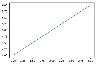
import numpy as np
import matplotlib.pyplot as plt

# 线性图
a = [1, 2, 3]
b = [4, 5, 6]
plt.plot(a, b)
plt.show()

import numpy as np
import matplotlib.pyplot as plt

# 线性图
x = np.linspace(0.0, 5.0)
y1 = np.sin(np.pi*x)
y2 = np.sin(np.pi*2*x)
plt.plot(x, y1,'b--', label='sin(pi*x)')
plt.ylabel('y1 value')
plt.plot(x, y2,'r--', label='sin(pi*2x)')
plt.ylabel('y2 value')
plt.xlabel('x value')
plt.title('this is a x-y value')
plt.legend()
plt.show()

import numpy as np
import matplotlib.pyplot as plt

# subplot 子图
x = np.linspace(0.0, 5.0)
y1 = np.sin(np.pi*x)
y2 = np.sin(np.pi*2*x)

# 子图一(‘2, 1, 1’ 等同于‘211’ 表示 两行一列第一个图)
plt.subplot(2, 1, 1)
plt.plot(x, y1, 'b--')
plt.ylabel('y1')
plt.xlabel('x')
#(‘2, 1, 2’ 等同于‘212’表示 两行一列第二个图)
plt.subplot(212)
plt.plot(x, y2, 'r--')
plt.ylabel('y2')
plt.xlabel('x')
plt.show()

# 子图二(‘2, 2’ 表示两行两列)
figure, ax = plt.subplots(2, 2)
ax[0][0].plot(x, y1)
ax[0][1].plot(x, y2)
# 此处只填充了 ax[0][0]、ax[0][1],ax[1][0]、ax[1][1] 未填充
plt.show()

import numpy as np
import pandas as pd
import matplotlib.pyplot as plt

# MatPlotLib-直方图
s = pd.Series(np.random.randn(1000))
# 直方图(rwidth 为宽度,bins 为分割区间,默认10)
plt.hist(s, rwidth=0.9, bins=30)
plt.show()

import numpy as np
import pandas as pd
import matplotlib.pyplot as plt

# MatPlotLib-密度图
s = pd.Series(np.random.randn(1000))
# 密度图
s.plot(kind='kde')
plt.show()

import numpy as np
import pandas as pd
import matplotlib.pyplot as plt

# pandas 的 Series 绘图
s1 = pd.Series(np.random.randn(1000)).cumsum()
s1.plot(kind='line', grid=True, label='s1', title='this is Series line')
plt.legend()
plt.show

import numpy as np
import pandas as pd
import matplotlib.pyplot as plt

# pandas 的 Series 绘图
s1 = pd.Series(np.random.randn(1000)).cumsum()
s2 = pd.Series(np.random.randn(1000)).cumsum()
s1.plot(kind='line', label='s1')
s2.plot(label='s2')
plt.legend()
plt.show()

# pandas 的 Series 绘图 - 子图
s1 = pd.Series(np.random.randn(1000)).cumsum()
s2 = pd.Series(np.random.randn(1000)).cumsum()
fig, ax = plt.subplots(2, 1)
ax[0].plot(s1)
ax[1].plot(s2)
plt.show()

# pandas 的 Series 绘图 - 子图
s1 = pd.Series(np.random.randn(1000)).cumsum()
s2 = pd.Series(np.random.randn(1000)).cumsum()
fig, ax =plt.subplots(2, 1)
s1[0: 10].plot(ax=ax[0], kind='bar')
s2.plot(ax=ax[1])
plt.show()

DataFrame plotting
DataFrame.plot
import numpy as np
import pandas as pd
import matplotlib.pyplot as plt

# pandas 的 DataFrame 绘图
df = pd.DataFrame(
    np.random.randint(1, 10, 40).reshape(10, 4),
    columns=['A', 'B', 'C', 'D']
)
df.plot()
plt.show()

# 按行(index)画图
df.iloc[5].plot()
plt.show()

# 按行(index)画图
for i in df.index:
    df.iloc[i].plot(label=str(i))
plt.legend()
plt.show()
# 同上
df.T.plot()
plt.show()

# 按列(columns)画图
for i in df.columns:
    df[i].plot(label=str(i))
plt.legend()
plt.show()

import numpy as np
import pandas as pd
import matplotlib.pyplot as plt
import seaborn as sns

s1 = pd.Series(np.random.randn(1000))
# pandas 直方图
plt.hist(s1)

# pandas 密度图
s1.plot(kind='kde')

# Seaborn-直方图和密度图
sns.distplot(s1, rug=True)

# Seaborn-密度图
sns.kdeplot(s1)

import numpy as np
import pandas as pd
import matplotlib.pyplot as plp
import seaborn as sns

# 使用 Seaborn 生成测试数据
df1 = sns.load_dataset('flights')
df = df1.pivot(index='month', columns='year', values='passengers')
load_dataset 为 Seaborn 提供的测试数据的获取方法(需要网络)。
数据地址:seaborn-data
# Seaborn-热力图
sns.heatmap(df)

# pandas-曲线图�
df.plot()

# pandas-柱状图
s.plot(kind='bar')

# Seaborn-柱状图
s = df.sum()
sns.barplot(x=s.index, y=s.values)

Style control
设置当前风格设置:seaborn.set_style
查看当前风格设置:seaborn.axes_style
更改当前图利属性:seaborn.set_context
查看当前图利属性:seaborn.plotting_context
取消个性化设置 seaborn.set
# Seaborn 绘图风格
style = ['darkgrid', 'dark', 'white', 'whitegrid', 'ticks']
# set_style 设置当前风格设置 第二个参数可进行个性化设置
sns.set_style(style[3])
# 查看当前风格设置
sns.axes_style()

# 更改当前图利属性
context = ['paper', 'notebook', 'talk', 'poster']
sns.set_context('paper')
# 查看当前图利属性
sns.plotting_context()
Color palettes
Choosing color palettes
查看当前色板(RGB):seaborn.color_palette
设置当前色板(RGB):seaborn.set_palette
# 查看当前色板(RGB)
sns.color_palette()

# 默认色板
pal_style = ['deep', 'muted', 'pastel', 'bright', 'dark', 'colorblind']

# 显示当前色板(RGB)
sns.palplot(sns.color_palette(pal_style[0]))

# 设置色板
sns.set_palette()

# 设置临时风格(with 语句外会恢复默认色板)
with sns.color_palette('dark'):
    sinplot() # 绘图方法

# 定义自定义色板('hls' 为固定值,8 表示生成8种颜色)
sns.color_palette('hls', 8)
sns.color_palette([(0.1, 0.2, 0.3), (...)])
以股票市场为例从 数据获取-导入-分析-可视化 完整流程
获取yahoo 股票数据:pandas-datareader
# anaconda 安装 pandas-datareader
conda install -c anaconda pandas-datareader数据获取的方法:
ChanMenglin/DataScience is a public repo on GitHub by ChanMenglin. Data-Science(数据科学).
It declares no license on GitHub. Public does not mean open source: without a license, nobody is granted the right to reuse it.
Its maker has not tagged a system, so it is unknown here. Its README says what it needs.
Open "Take it" on its page: Take My Repo writes an install plan for your machine and hands it to your AI agent (Claude Code, Codex or Cursor), which asks you before each step. Take My Repo has not tested it on any machine.
Its last change on GitHub was on 2021-08-03. Take My Repo does not judge from that whether it is maintained.
Nobody has reviewed it on Take My Repo yet, which says nothing about its quality.
Official repository for Spyder - The Scientific Python Development Environment
Bring data to life with SVG, Canvas and HTML. :bar_chart::chart_with_upwards_trend::tada:
Apache Superset is a Data Visualization and Data Exploration Platform
12 weeks, 26 lessons, 52 quizzes, classic Machine Learning for all
Visual analysis and diagnostic tools to facilitate machine learning model selection.