
Java-Solutions-TCS-IPA-Questions
Java Solutions of TCS IPA exam. 35 marks and 15 marks questions are solved.
- 564
- Java
- 3 y ago
Matplotlib Pyplot Cheat Sheet 2023
Repo mpolinowski/python-matplotlib-2023, read from GitHub 1 min ago. mpolinowski has not joined Take My Repo.
mpolinowski/python-matplotlib-2023 is a public repo on GitHub by mpolinowski. Matplotlib Pyplot Cheat Sheet 2023. It declares no license on GitHub. Public does not mean open source: without a license, nobody is granted the right to reuse it. It is written mainly in Jupyter Notebook, has 4 stars and last changed on 2023-05-06. Nobody has reviewed it on Take My Repo yet, which says nothing about its quality. Read from GitHub on 2026-11-19.
import matplotlib.pyplot as plt
import numpy as np
from numpy.random import randint
x = np.arange(-10,10)
y = x**2
a = np.linspace(0,10,20)
b = a**5+a**2
np.random.seed(42)
xz = 4 + np.random.normal(0, 2, 24)
yz = 4 + np.random.normal(0, 2, len(xz))
rand = randint(1,50,20)
name_array = ['First Dataset', 'Second Dataset', 'Third Dataset']
x_array = [rand, rand-15, rand**(1/2)]
y_array = [rand**(3/4), rand**2, rand**(2/3)]
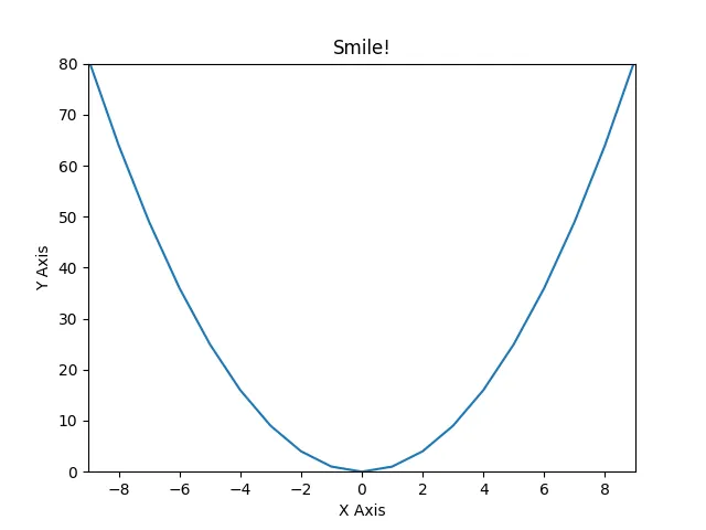
plt.plot(x, y)
plt.xlabel('X Axis')
plt.ylabel('Y Axis')
plt.xlim(-9, 9)
plt.ylim(0, 80)
plt.title('Smile!')
plt.savefig('assets/Matplotlib_Pyplot_Cheat_Sheet_01.webp')

figure = plt.figure(figsize=(10,10))
# add_axes[(lower left corner x,y), width&height of plot inside figure [0-1]]
axes = figure.add_axes([0,0,1,0.2])
# start plot at 0,0 and use 100% width but only 20% height
axes.plot(x, y)

fig = plt.figure(figsize=(10,5))

ax_xy = fig.add_axes([0.1,0.1,0.5,0.8])
ax_xy.plot(x, y)
ax_xy.set_xlim(-10, 10)
ax_xy.set_ylim(0, 100)
ax_xy.set_xlabel('X Axis')
ax_xy.set_ylabel('Y Axis')
ax_xy.set_title('A/B Plot Title')

ax_ab_sub1 = fig.add_axes([0.68,0.6,0.3,0.3])
ax_ab_sub1.plot(a, b)
ax_ab_sub1.set_xlim(3,6)
ax_ab_sub1.set_ylim(0, 5000)
ax_ab_sub1.set_xlabel('A Axis')
ax_ab_sub1.set_ylabel('B Axis')
ax_ab_sub1.set_title('X/Y Plot Title')

ax_ab_sub2 = fig.add_axes([0.68,0.1,0.3,0.3])
ax_ab_sub2.plot(a, b)
ax_ab_sub2.set_xlim(7,10)
ax_ab_sub2.set_ylim(25000, 75000)
ax_ab_sub2.set_xlabel('A Axis')
ax_ab_sub2.set_ylabel('B Axis')
ax_ab_sub2.set_title('X/Y Plot Title')

fig.savefig('assets/Matplotlib_Pyplot_Cheat_Sheet_03.webp', bbox_inches='tight')

fig, axes = plt.subplots(figsize=(10,5), nrows=1, ncols=2)

axes[0].plot(x, y)
axes[1].plot(a, b)

plt.savefig('assets/Matplotlib_Pyplot_Cheat_Sheet_04.webp')

fig, axes = plt.subplots(figsize=(10, 5), nrows=2, ncols=2)

fig.suptitle('Plot Title')

axes[0][0].plot(x, y)
axes[0][0].set_xlabel('X Axis')
axes[0][0].set_ylabel('Y Axis')
axes[0][0].set_title('X/Y Title')

axes[0][1].plot(a, b)
axes[0][1].set_xlabel('A Axis')
axes[0][1].set_ylabel('B Axis')
axes[0][1].set_title('A/B Title')

axes[1][0].plot(a, b)
axes[1][0].set_xlabel('A Axis')
axes[1][0].set_ylabel('B Axis')
axes[1][0].set_title('A/B Title')

axes[1][1].plot(x, y)
axes[1][1].set_xlabel('X Axis')
axes[1][1].set_ylabel('Y Axis')
axes[1][1].set_title('X/Y Title')

fig.subplots_adjust(
    left=None,
    bottom=None,
    right=None,
    top=None,
    wspace=0.5,
    hspace=1
)

plt.savefig('assets/Matplotlib_Pyplot_Cheat_Sheet_05.webp')

fig, axes = plt.subplots(figsize=(10,5), nrows=3, ncols=1)

fig.suptitle('I am Scattered')

counter = 0

for ax in axes:
    ax.plot(
        x_array[counter],
        y_array[counter],
        color='g',
        marker='P',
        linestyle='None'
    )
    ax.set_title(name_array[counter])
    counter += 1

plt.tight_layout()

plt.savefig('assets/Matplotlib_Pyplot_Cheat_Sheet_06.webp')

fig = plt.figure(figsize=(12,8))

ax = fig.add_axes([0,0,1,1])

ax.plot(a, a**(4/3), label="x, x**4/3")
ax.plot(a, a, label="x, x")
ax.plot(a, a**(2/3), label="x, x**2/3")
ax.plot(a, a**(1/2), label="x, x**1/2")

ax.legend(loc='upper left')

plt.savefig('assets/Matplotlib_Pyplot_Cheat_Sheet_07.webp', bbox_inches='tight')

fig = plt.figure(figsize=(12,8))

ax = fig.add_axes([0,0,1,1])

ax.plot(a, a**(4/3), label="x, x**4/3")
ax.plot(a, a, label="x, x")
ax.plot(a, a**(2/3), label="x, x**2/3")
ax.plot(a, a**(1/2), label="x, x**1/2")

ax.legend(loc=(1.1, 0.9))
plt.tight_layout()

plt.savefig('assets/Matplotlib_Pyplot_Cheat_Sheet_08.webp', bbox_inches='tight')

fig = plt.figure(figsize=(12,8))

ax = fig.add_axes([0,0,1,1])

ax.plot(
    a,a,
    color='dodgerblue',
    linewidth='5',
    label="a, a"
)
ax.plot(
    a,(a**(3/2)+b**(1/2)),
    color='#fd18d9',
    linestyle='dashed',
    marker='h',
    markersize=16,
    markerfacecolor='lightseagreen',
    markeredgewidth=3,
    markeredgecolor='fuchsia',
    label="a,(a**(3/2)+b**(1/2)"
)
# supported marker styles are: ".", ",", "o", "v", "^", "<", ">", "1", "2", "3", "4", "8", "s", "p", "P", "*", "h", "H", "+", "x", "X", "D", "d", "|", "_"
# supported line styles are '-', '--', '-.', ':', 'None', ' ', '', 'solid', 'dashed', 'dashdot', 'dotted'

ax.legend()

plt.savefig('assets/Matplotlib_Pyplot_Cheat_Sheet_09.webp', bbox_inches='tight')

fig, ax = plt.subplots(1, 2, figsize=(12,8))

ax[0].plot(a,a,label="a, a")
ax[0].plot(a,(a**(3/2)+b**(1/2)),label="a,(a**(3/2)+b**(1/2)")
ax[0].grid(True)
ax[0].legend()
ax[0].set_title('Linear Scale')

ax[1].plot(a,a,label="a, a")
ax[1].plot(a,(a**(3/2)+b**(1/2)),label="a,(a**(3/2)+b**(1/2)")
ax[1].set_yscale('log')
ax[1].grid(True)
ax[1].legend()
ax[1].set_title('Log Scale')

plt.savefig('assets/Matplotlib_Pyplot_Cheat_Sheet_10.webp', bbox_inches='tight')

np.random.seed(42)
N = 40
theta = np.linspace(0.0, 2*np.pi, N, endpoint=False)
radii = 10*np.random.rand(N)
width = np.pi/4*np.random.rand(N)
colours = plt.cm.winter(radii/10)
plt.figure(figsize=(10,10))
ax = plt.subplot(1,1,1, projection='polar')
ax.bar(
    theta,
    radii,
    width=width,
    bottom=0,
    color=colours,
    alpha=0.7
)
ax.set_title('Polar Bar Chart')

plt.savefig('assets/Matplotlib_Pyplot_Cheat_Sheet_27.webp', bbox_inches='tight')

radii2 = np.arange(0, 2, 0.01)
theta2 = 2*np.pi*radii2
plt.figure(figsize=(10,10))

ax = plt.subplot(111, projection='polar')
ax.plot(theta2, radii2, color='mediumspringgreen')
ax.set_rmax(2)
ax.set_rticks([0, 0.5, 1.5])
ax.set_title('Polar Line Chart')

plt.savefig('assets/Matplotlib_Pyplot_Cheat_Sheet_28.webp', bbox_inches='tight')

np.random.seed(42)
N = 200
radii3 = 3*np.random.rand(N)
theta3 = 2*np.pi*np.random.rand(N)
area = 50*2*np.pi*radii3**2
colours = theta3
fig = plt.figure(figsize=(10,10))

ax = fig.add_subplot(111, projection='polar')
plot = ax.scatter(theta3, radii3, c=colours, s=area, cmap='spring', alpha=0.8)

plt.savefig('assets/Matplotlib_Pyplot_Cheat_Sheet_29.webp', bbox_inches='tight')

fig, ax1 = plt.subplots(figsize=(12,8))

ax1.plot(a,(a**(3/2)+b**(1/2)), lw=2, color='dodgerblue')
ax1.set_ylabel(r"area $(m^2)$", fontsize=18, color='dodgerblue')
for label in ax1.get_yticklabels():
    label.set_color('dodgerblue')

ax2 = ax1.twinx()
ax2.plot(a,(a**(4/3)+b**(2/3)), lw=2, color='mediumorchid')
ax2.set_ylabel(r"volume $(m^3)$", fontsize=18, color='mediumorchid')
for label in ax2.get_yticklabels():
    label.set_color('mediumorchid')

plt.savefig('assets/Matplotlib_Pyplot_Cheat_Sheet_11.webp', bbox_inches='tight')

fig, ax = plt.subplots(figsize=(12,8))
ax.set_title('Plot Annotation')
ax.plot(x**2+x, x**3)

plt.annotate(
    text='Wooh!',
    xy=(0, 0),
    xycoords='data',
    xytext=(0.3, 0.3),
    textcoords='axes fraction',
    va='top', ha='left',
    arrowprops=dict(facecolor='tomato', shrink=0),
    color='royalblue',
    weight='heavy'
)

plt.savefig('assets/Matplotlib_Pyplot_Cheat_Sheet_12.webp', bbox_inches='tight')

plt.pie(d)
plt.title('Pie Chart')

plt.savefig('assets/Matplotlib_Pyplot_Cheat_Sheet_13.webp', bbox_inches='tight')

d = [1, 2, 5, 7, 5, 7, 2]
e = (0., 0.05, 0.05, 0., 0., 0., 0.)
pie_labels = ['Cupim', 'Velit', 'Nulla', 'Leberkas', 'Cillum', 'Incididunt', 'Fugiat']
colors = plt.get_cmap('cool')(np.linspace(0.2, 0.7, len(d)))

fig, ax = plt.subplots(figsize=(10,10))

wedges, texts, autotexts = ax.pie(
    d,
    autopct='%1.1f%%',
    pctdistance=0.6,
    colors=colors,
    labels = pie_labels,
    labeldistance=1.15,
    explode=e,
    startangle=130,
    wedgeprops={"linewidth": 1, "edgecolor": "white"},
    shadow=True
)

plt.setp(autotexts, size=13, color='white')
plt.setp(texts, size=14, color='darkslategray')
ax.set_title('Andouille Biltong Voluptate')

# ax.set(xlim=(0, 8), xticks=np.arange(1, 8),
#        ylim=(0, 8), yticks=np.arange(1, 8))

fig.savefig('assets/Matplotlib_Pyplot_Cheat_Sheet_14.webp', bbox_inches='tight')

fig, ax = plt.subplots(figsize=(10,10))
size = 0.3

values = np.array([[88,44], [22,77], [99,11]])
value_sum = values.sum(axis=1)
value_flat = values.flatten()

value_sum_labels = ['Cupim', 'Velit', 'Nulla']
value_flat_labels = ['Leberkas', 'Cillum', 'Incididunt', 'Fugiat', 'Kielbasa', 'Picanha']

cmap = plt.get_cmap('cool')
outer_colors = cmap(np.linspace(0.1, 0.4, len(value_sum)))
inner_colors = cmap(np.linspace(0.5, 0.9, len(value_sum)))

wedges, texts, autotexts = ax.pie(
    value_sum,
    radius = 1,
    colors = outer_colors,
    labels = value_sum_labels,
    autopct='%1.1f%%',
    pctdistance=0.8,
    wedgeprops = {
        'linewidth': 1,
        'width': size,
        'edgecolor': "white"
    }
)

plt.setp(autotexts, size=13, color='white')
plt.setp(texts, size=14, color='darkslategray')

wedges2, texts2, autotexts2 = ax.pie(
    value_flat,
    radius = 1 - size,
    colors = inner_colors,
    labels = value_flat_labels,
    labeldistance=0.22,
    autopct='%1.1f%%',
    pctdistance=0.8,
    wedgeprops = {
        'linewidth': 1,
        'width': size,
        'edgecolor': "white"
    }
)

plt.setp(autotexts2, size=13, color='white')
plt.setp(texts2, size=10, color='darkslategray')

ax.set_title('Et Donut Burgdoggen Exercitatione')

fig.savefig('assets/Matplotlib_Pyplot_Cheat_Sheet_25.webp', bbox_inches='tight')

measurements = [
    '323 ppm Cupim',
    '72 ppm Velit',
    '112 ppm Nulla',
    '224 ppm Cillum',
    '56 ppm Incididunt'
]

results = [float(x.split(' ')[0]) for x in measurements]
substances = [str(x.split(' ')[-1]) for x in measurements]

def percentage(pct, values):
    absolute = int(pct/100. * np.sum(values))
    return '{:.1f}%\n({:d} ppm)'.format(pct, absolute)
fig, ax = plt.subplots(figsize=(10,10))

wedges, texts, autotexts = ax.pie(
    result,
    autopct = lambda pct: percentage(pct, results)
)

ax.legend(
    wedges,
    substances,
    title = 'Measurement',
    bbox_to_anchor = (0.5, 0, 0.5, 1)
)

plt.setp(autotexts, size=13, color='white')
plt.setp(texts, size=14, color='darkslategray')

fig.savefig('assets/Matplotlib_Pyplot_Cheat_Sheet_26.webp', bbox_inches='tight')

plt.scatter(xz,yz)
plt.title('Scatter Plot')

plt.savefig('assets/Matplotlib_Pyplot_Cheat_Sheet_15.webp', bbox_inches='tight')

# size and color:
sizes = np.random.uniform(15, 80, len(xz))
colors = np.random.uniform(15, 80, len(xz))

fig, ax = plt.subplots()
ax.scatter(xz, yz, s=sizes, c=colors, vmin=0, vmax=100)
ax.set_title('Scatter Chart')
ax.set(xlim=(0, 8), xticks=np.arange(1, 8),
       ylim=(0, 8), yticks=np.arange(1, 8))

fig.savefig('assets/Matplotlib_Pyplot_Cheat_Sheet_16.webp', bbox_inches='tight')

plt.bar(a,b)
plt.title('Bar Chart')

plt.savefig('assets/Matplotlib_Pyplot_Cheat_Sheet_17.webp', bbox_inches='tight')

fig, ax = plt.subplots()

ax.bar(x, y, width=0.6, edgecolor="white", linewidth=0.7)
ax.set_title('Bar Chart')
ax.set(xlim=(0, 10), xticks=np.arange(1, 10),
       ylim=(0, 110))

plt.savefig('assets/Matplotlib_Pyplot_Cheat_Sheet_18.webp', bbox_inches='tight')

bins = np.linspace(0,20,20)

plt.hist(
    y_array[0],
    bins=bins,
    rwidth=0.8
)
plt.title('Histogram')

plt.savefig('assets/Matplotlib_Pyplot_Cheat_Sheet_19.webp', bbox_inches='tight')

fig, ax = plt.subplots()
ax.hist(xs, bins=8, linewidth=0.5, edgecolor="white")
ax.set_title('Histogram')
ax.set(xlim=(22, 33), xticks=np.arange(22, 33),
        ylim=(0, 20), yticks=np.linspace(0, 18, 9))

plt.savefig('assets/Matplotlib_Pyplot_Cheat_Sheet_20.webp', bbox_inches='tight')

# generate two datasets - one with a standard deviation of 1 the other with std=2
data = [np.random.normal(0, std, 100) for std in range(1,3)]
plt.boxplot(data, vert=True, patch_artist=True)
plt.title('STD Boxplot')
plt.savefig('assets/Matplotlib_Pyplot_Cheat_Sheet_24.webp', bbox_inches='tight')

fig, ax = plt.subplots()

ax.fill_between(x, y, y**(1/2), alpha=.5, linewidth=0)
ax.plot(x, (y + y**(1/2))/2, linewidth=2)
ax.set_title('Fill Between Chart')
ax.set(xlim=(-10, 10), xticks=np.arange(-10, 10),
        ylim=(0, 100))

plt.savefig('assets/Matplotlib_Pyplot_Cheat_Sheet_21.webp', bbox_inches='tight')

from matplotlib.patches import Polygon
def f(x):
    return (x-3) * (x-4) * (x-7) + 77

a, b = 2, 9
x = np.linspace(0,10)
y = f(x)
fig, ax = plt.subplots(figsize=(12,8))

ax.plot(x, y, color='fuchsia', linewidth=2)
ax.set_title('Integral of the Area under the Curve')
ax.set_xlabel('X')
ax.set_ylabel('Y')
ax.spines['right'].set_visible(False)
ax.spines['top'].set_visible(False)

# select section of curve
ax.set_ylim(bottom=0)
ix = np.linspace(a,b)
iy = f(ix)
verts = [(a, 0), *zip(ix,iy), (b, 0)]
ax.set_xticks((a,b))
ax.set_xticklabels(('a','b'))
ax.set_yticks((f(a),f(b)))
ax.set_yticklabels(('f(a)','f(b)'))

# draw polygon under selection
poly = Polygon(verts, facecolor='dodgerblue', edgecolor='fuchsia')
ax.add_patch(poly)
# annotate
ax.text(
    0.5*(a+b), 30,
    r'$\int_a^b f(x)\mathrm{d}x$',
    color='white',
    fontsize='xx-large'
)

plt.savefig('assets/Matplotlib_Pyplot_Cheat_Sheet_30.webp', bbox_inches='tight')

# i am not sure if `from matplotlib.patches import Polygon`
# has a method to calculate the area of a polygon?
# but it does work with `pip install shaply`:
from shapely.geometry import Polygon
polygon = Polygon(verts)
polygon.area
# 571.1428571428572
np.random.seed(42)
n = 100
rng = np.random.default_rng()
xs = rng.uniform(23, 32, n)
ys = rng.uniform(0, 100, n)
zs = rng.uniform(-50, -25, n)
fig = plt.figure(figsize=(10,10))
ax = plt.axes(projection='3d')
ax.set_title('3D Line Chart')
ax.plot3D(xs, ys, zs)

plt.savefig('assets/Matplotlib_Pyplot_Cheat_Sheet_22.webp', bbox_inches='tight')

fig, ax = plt.subplots(figsize=(12,8), subplot_kw={"projection": "3d"})

ax.scatter(xs, ys, zs)
ax.set_title('3D Scatterplot')
ax.set(xticklabels=[],
       yticklabels=[],
       zticklabels=[])

fig.savefig('assets/Matplotlib_Pyplot_Cheat_Sheet_23.webp', bbox_inches='tight')

from matplotlib.animation import FuncAnimation
from psutil import cpu_percent
from datetime import datetime
usage = []
cpu_use = cpu_percent()
usage.append((datetime.utcnow(), cpu_use))
usage
#[(datetime.datetime(2023, 5, 6, 8, 43, 39, 187158), 13.3),
#  (datetime.datetime(2023, 5, 6, 8, 43, 40, 67655), 12.2),
#  (datetime.datetime(2023, 5, 6, 8, 43, 40, 744222), 14.7)]
plt.plot(*zip(*usage), color='mediumspringgreen')
plt.title('CPU Usage in Percent')
plt.savefig('assets/Matplotlib_Pyplot_Cheat_Sheet_31.webp', bbox_inches='tight')

%matplotlib notebook
# only display 200 data points
frame_len = 200
data_points=[]

fig = plt.figure(figsize=(8,5))
fig.suptitle('Realtime CPU Usage [%]')

plt.ylim(1,100)
plt.tight_layout()

def animation(i):
    data_points.append((datetime.utcnow(), cpu_percent()))

    if len(y) <= frame_len:
        plt.cla()
        plt.plot(*zip(*data_points), color='mediumspringgreen', label='CPU Usage [%]')
    else:
        plt.cla()
        plt.plot(data_points[-frame_len:],color='mediumspringgreen', label='CPU Usage [%]')

anime = FuncAnimation(plt.gcf(), animation, interval=1000)

from scipy import constants as sc
c_vac = sc.speed_of_light
mass = np.linspace(0,100)

def energy_conversion(mass):
    return mass * c_vac**2

energy = energy_conversion(mass)
fig = plt.figure(figsize=(8,5))
fig.suptitle('Mass to Energy Conversion')

plt.xlabel('Mass')
plt.ylabel('Energy')
plt.legend()
plt.plot(mass, energy, label='E = m*c²')
fig = plt.figure(figsize=(8,5))
fig.suptitle('Mass to Energy Conversion')

ax = fig.add_axes([0,0,1,1])

ax.plot(
    mass,energy,
    color='#fd18d9',
    linestyle='dashed',
    marker='h',
    markersize=8,
    markerfacecolor='lightseagreen',
    markeredgewidth=2,
    markeredgecolor='fuchsia',
    label="E = m*c²"
)

ax.legend(loc='upper left')
ax.set_xlabel('Mass')
ax.set_ylabel('Energy')

plt.savefig('assets/Matplotlib_Pyplot_Cheat_Sheet_33.webp', bbox_inches='tight')

fig, ax = plt.subplots(1, 2, figsize=(12,8))

ax[0].plot(
    mass,energy,
    color='lightseagreen',
    linestyle='dashed',
    label="E = m*c²"
)
ax[0].legend()
ax[0].set_xlabel('Mass')
ax[0].set_ylabel('Energy')
ax[0].grid(True)
ax[0].set_title('E = m*c²')

ax[1].plot(
    mass,energy,
    color='dodgerblue',
    linestyle='dashed',
    label="E = m*c²"
)
ax[1].set_yscale('log')
ax[1].grid(True)
ax[1].legend()
ax[1].set_xlabel('Mass')
ax[1].set_ylabel('Energy')
ax[1].set_title('E = m*c² (log)')

plt.savefig('assets/Matplotlib_Pyplot_Cheat_Sheet_34.webp', bbox_inches='tight')

mpolinowski/python-matplotlib-2023 is a public repo on GitHub by mpolinowski. Matplotlib Pyplot Cheat Sheet 2023.
It declares no license on GitHub. Public does not mean open source: without a license, nobody is granted the right to reuse it.
Its maker has not tagged a system, so it is unknown here. Its README says what it needs.
Open "Take it" on its page: Take My Repo writes an install plan for your machine and hands it to your AI agent (Claude Code, Codex or Cursor), which asks you before each step. Take My Repo has not tested it on any machine.
Its last change on GitHub was on 2023-05-06. Take My Repo does not judge from that whether it is maintained.
Java Solutions of TCS IPA exam. 35 marks and 15 marks questions are solved.
Nobody has reviewed it on Take My Repo yet, which says nothing about its quality.
A list of useful payloads and bypass for Web Application Security and Pentest/CTF
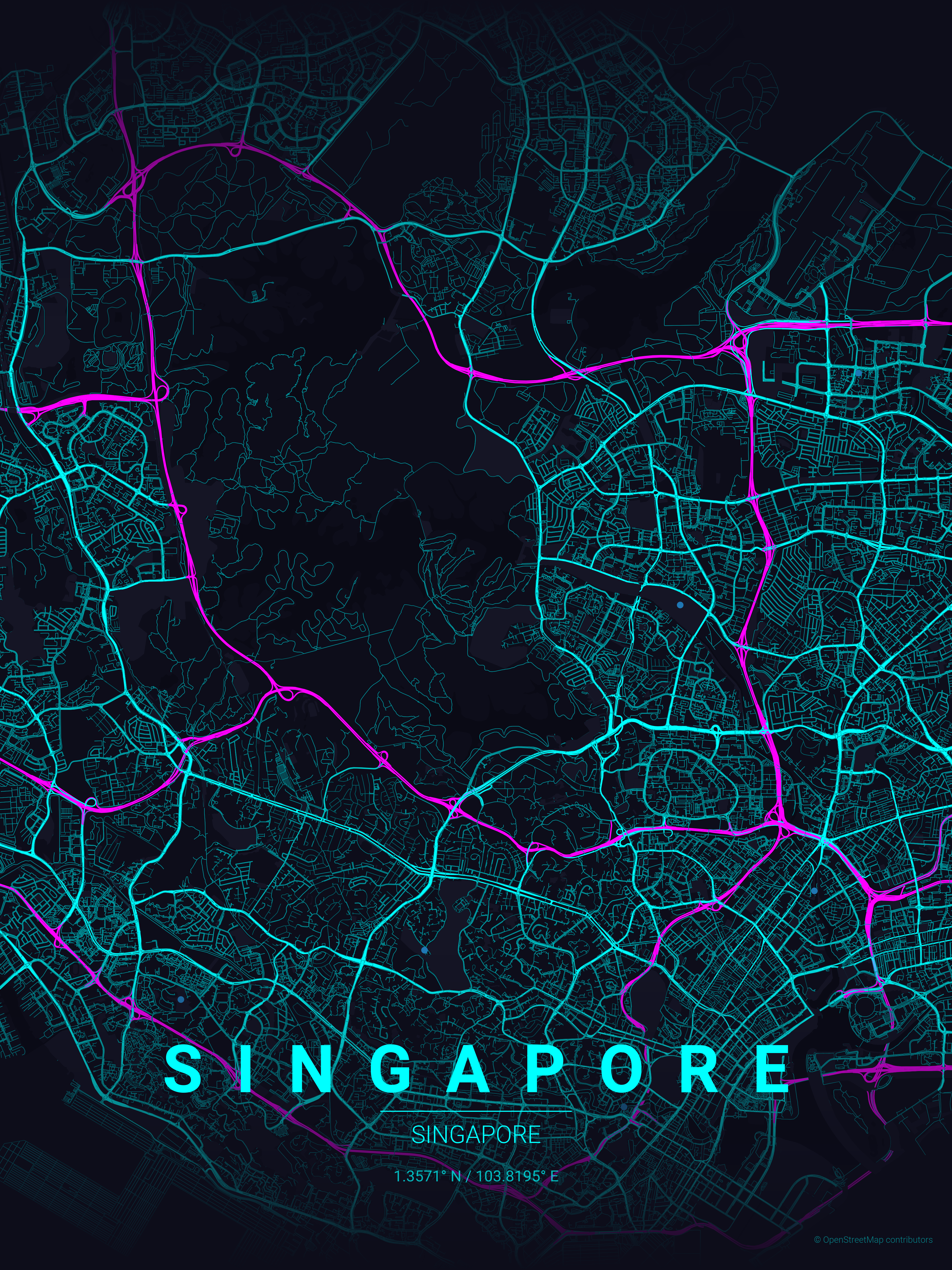
Transform your favorite cities into beautiful, minimalist designs. MapToPoster lets you create and export visually striking map posters with code.
All logos of teams in the top 25 European (UEFA) leagues. Seasons 2021/22 to 2026/27.
Matplotlib is an amazing visualization library in Python for 2D plots of arrays. Matplotlib is a multi-platform data visualization library built on NumPy arrays and designed to work with the broader SciPy stack. It was introduced by John Hunter in the year 2002. One of the greatest benefits of visualization is that it allows us visual access to huge amounts of data in easily digestible visuals. Ma
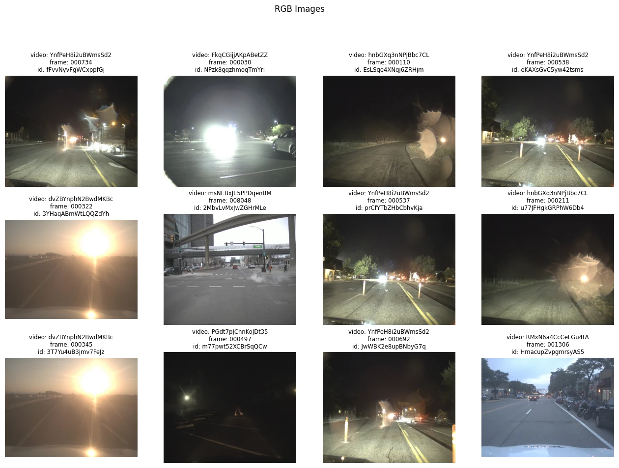
Using YOLOv8 to build a Object Classifier/Tracker for RBG/Thermal Cameras