moead-in-python
A comprehensive Python implementation of MOEA/D (Multiobjective Evolutionary Algorithm based on Decomposition), a state-of-the-art algorithm for solving multiobjective optimization problems. This implementation is based on the seminal work by Zhang and Li (2007).
- 2
- MIT
- 13 mo ago
Repo smkalami/moead-in-python, read from GitHub 4 h ago. smkalami has not joined Take My Repo.
In short
smkalami/moead-in-python is a public repo on GitHub by smkalami. A comprehensive Python implementation of MOEA/D (Multiobjective Evolutionary Algorithm based on Decomposition), a state-of-the-art algorithm for solving multiobjective optimization problems. This implementation is based on the seminal work by Zhang and Li (2007). It declares the MIT license on GitHub. It is written mainly in Python, has 2 stars and last changed on 2025-10-21. Nobody has reviewed it on Take My Repo yet, which says nothing about its quality. Read from GitHub on 2026-11-22.
MOEA/D: Multiobjective Evolutionary Algorithm based on Decomposition
A comprehensive Python implementation of MOEA/D (Multiobjective Evolutionary Algorithm based on Decomposition), a state-of-the-art algorithm for solving multiobjective optimization problems. This implementation is based on the seminal work by Zhang and Li (2007).
🧠 What is MOEA/D?
The Challenge of Multiobjective Optimization
In real-world problems, we often need to optimize multiple conflicting objectives simultaneously:
- Engineering Design: Minimize cost vs. maximize performance
- Portfolio Optimization: Maximize return vs. minimize risk
- Machine Learning: Minimize error vs. minimize complexity
Unlike single-objective optimization, there's no single "best" solution. Instead, we seek a Pareto front - a set of trade-off solutions where improving one objective requires worsening another.
MOEA/D's Innovation
Traditional algorithms like NSGA-II tackle multiobjective problems directly using dominance relationships. MOEA/D takes a different approach:
🔄 Key Insight: Decompose the complex multiobjective problem into many simpler single-objective subproblems and solve them cooperatively.
Think of it as teamwork: Each "specialist" (subproblem) focuses on one region of the Pareto front, while sharing information with neighboring specialists to collectively cover the entire front efficiently.
Why MOEA/D?
✅ Computationally Efficient: Lower complexity than dominance-based methods
✅ Natural Diversity: Weight vectors ensure uniform distribution along Pareto front
✅ Scalable: Handles 2, 3, or many objectives effectively
✅ Flexible: Easy to integrate different decomposition methods
✅ Proven Performance: Extensively validated in literature
🏗️ Project Structure
MOEA-D in Python/
├── moead.py              # Core MOEA/D algorithm implementation
├── test_problems.py      # Standard benchmark functions (ZDT, DTLZ, etc.)
├── example.py            # Simple interface function + problem solver
├── images/               # Example results and visualizations
│   └── moead_result_for_zdt1.png
├── requirements.txt      # Required Python packages
├── LICENSE              # MIT License
├── .gitignore           # Git ignore patterns
└── README.md            # This file
Core Components
MOEADclass: Main algorithm with customizable parameters- Decomposition methods: Weighted Sum and Tchebycheff approaches
- Evolutionary operators: Simulated Binary Crossover (SBX) and Polynomial Mutation
- Test suite: Standard problems for benchmarking and validation
- Simple interface: Easy-to-use functions for quick problem solving
🚀 Quick Start
Installation
# Clone or download the project files
# Install dependencies
pip install -r requirements.txt
Requirements: numpy, scipy, matplotlib
30-Second Example
from example import run_moead_simple
from test_problems import TestProblems

# Solve ZDT1 benchmark problem
results = run_moead_simple(
    objective_function=TestProblems.zdt1,
    n_objectives=2,
    n_variables=10,
    bounds=[(0, 1)] * 10,
    population_size=100,
    max_generations=200,
    plot_title="ZDT1 Pareto Front"
)

# Results automatically plotted and returned
print(f"Found {len(results['objectives'])} Pareto optimal solutions!")
Example Output:
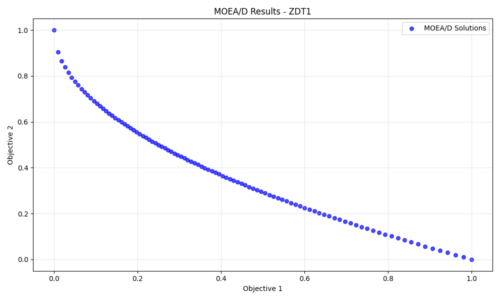
MOEA/D finds a well-distributed approximation of the ZDT1 Pareto front
For Your Custom Problem
import numpy as np
from example import run_moead_simple

# Define your multiobjective function
def my_problem(x):
    """Example: Portfolio optimization"""
    f1 = np.sum(x**2)                    # Risk (minimize)
    f2 = -np.sum(x * np.arange(1, len(x)+1))  # Return (maximize, so negate)
    return np.array([f1, f2])

# Solve it!
results = run_moead_simple(
    objective_function=my_problem,
    n_objectives=2,
    n_variables=5,
    bounds=[(-2, 2)] * 5,
    plot_title="Portfolio Optimization"
)
📊 Algorithm Details
Decomposition Methods
MOEA/D transforms the multiobjective problem using one of these approaches:
1. Weighted Sum
$$g^{ws}(x|\lambda) = \sum_{i=1}^{m} \lambda_i f_i(x)$$
- Pros: Simple, fast
- Cons: Cannot find solutions on non-convex Pareto fronts
- Use when: Pareto front is known to be convex
2. Tchebycheff (Recommended)
$$g^{te}(x|\lambda, z^\ast) = \max_{i} \lambda_i |f_i(x) - z_i^\ast|$$
- Pros: Handles any Pareto front shape (convex, non-convex, disconnected)
- Cons: Slightly more complex
- Use when: General-purpose optimization (default choice)
Algorithm Flow
- 🎯 Decomposition: Create $N$ uniformly distributed weight vectors $\lambda^1, \lambda^2, \ldots, \lambda^N$
- 🏘️ Neighborhoods: Group similar weight vectors as "neighbors"
- 🔄 Evolution: For each generation:
- Select parents from neighborhood
- Create offspring via crossover & mutation
- Update neighboring solutions if offspring improves them
- 📈 Result: Final population approximates the Pareto front
Key Parameters
| Parameter | Description | Typical Values |
|---|---|---|
population_size |
Number of subproblems ($N$) | $50\text{-}100$ (2 obj), $100\text{-}200$ (3+ obj) |
max_generations |
Evolution iterations | $200\text{-}500$ |
decomposition |
Decomposition method | 'tchebycheff' (recommended) |
neighborhood_size |
Cooperating subproblems ($T$) | $20$ (default) |
crossover_rate |
SBX probability ($p_c$) | $0.9$ (default) |
mutation_rate |
Polynomial mutation prob. ($p_m$) | $0.1$ (default) |
🛠️ Usage Examples
Method 1: Simple Interface (Recommended)
from example import run_moead_simple
import numpy as np

def engineering_design(x):
    """Minimize weight and maximize strength"""
    weight = np.sum(x**2)
    strength = -np.prod(x)  # Negative because we maximize
    return np.array([weight, strength])

results = run_moead_simple(
    objective_function=engineering_design,
    n_objectives=2,
    n_variables=4,
    bounds=[(0.1, 2.0)] * 4,
    population_size=100,
    max_generations=300,
    decomposition='tchebycheff',
    plot_title="Engineering Design Trade-off"
)

# Access results
pareto_front = results['objectives']
pareto_solutions = results['population']
Method 2: Direct API Usage
from moead import MOEAD
import numpy as np

def my_function(x):
    return np.array([x[0]**2, (x[0]-2)**2])

# Configure algorithm
moead = MOEAD(
    n_objectives=2,
    n_variables=1,
    population_size=50,
    bounds=[(-5, 5)],
    decomposition='tchebycheff'
)

# Run optimization
population, objectives = moead.optimize(my_function, max_generations=100)
Method 3: Benchmark Testing
from test_problems import TestProblems
from example import run_moead_simple

# Test on standard problems
problems = ['zdt1', 'zdt2', 'zdt3']

for prob_name in problems:
    problem_func = TestProblems.get_problem(prob_name)

    results = run_moead_simple(
        objective_function=problem_func,
        n_objectives=2,
        n_variables=10,
        bounds=[(0, 1)] * 10,
        plot_title=f"MOEA/D on {prob_name.upper()}"
    )

    print(f"{prob_name}: {len(results['objectives'])} solutions found")
📚 Included Test Problems
| Problem | Objectives | Variables | Pareto Front Characteristics |
|---|---|---|---|
| ZDT1 | 2 | 10 | Convex: $f_2 = 1 - \sqrt{f_1}$ |
| ZDT2 | 2 | 10 | Non-convex: $f_2 = 1 - f_1^2$ |
| ZDT3 | 2 | 10 | Disconnected with gaps |
| DTLZ1 | 3+ | 7+ | $m$-dimensional linear simplex |
| Schaffer | 2 | 1 | Simple convex for quick testing |
These problems are extensively used in multiobjective optimization research for benchmarking algorithms.
🔧 Customization & Tips
For Better Results
Choose the right decomposition:
- Use
'tchebycheff'for unknown or complex Pareto fronts - Use
'weighted_sum'only if you know the front is convex
- Use
Scale your problem appropriately:
- Population size: 50-100 for 2 objectives, 100-200 for 3+ objectives
- Generations: Start with 200, increase if convergence is poor
Normalize objectives if scales differ greatly:
def normalized_objectives(x):
    f1 = objective1(x) / 1000  # Scale down large values
    f2 = objective2(x) * 100   # Scale up small values
    return np.array([f1, f2])
Common Issues & Solutions
| Issue | Solution |
|---|---|
| Poor convergence | Increase max_generations or population_size |
| Uneven distribution | Use decomposition='tchebycheff' |
| Slow performance | Reduce population_size or use 'weighted_sum' |
| Memory issues | Reduce population_size |
📖 Learning More
- Zhang & Li (2007): Original paper - "MOEA/D: A multiobjective evolutionary algorithm based on decomposition"
- Examples in code: Run
example.pyfor comprehensive demonstrations
📄 License
MIT License - Feel free to use in your research and projects.
See LICENSE file for full details.
Questions
What is moead-in-python?
smkalami/moead-in-python is a public repo on GitHub by smkalami. A comprehensive Python implementation of MOEA/D (Multiobjective Evolutionary Algorithm based on Decomposition), a state-of-the-art algorithm for solving multiobjective optimization problems. This implementation is based on the seminal work by Zhang and Li (2007).
Is moead-in-python open source?
It declares the MIT license on GitHub.
Does moead-in-python run on macOS, Windows or Linux?
Its maker has not tagged a system, so it is unknown here. Its README says what it needs.
How do I install moead-in-python?
Open "Take it" on its page: Take My Repo writes an install plan for your machine and hands it to your AI agent (Claude Code, Codex or Cursor), which asks you before each step. Take My Repo has not tested it on any machine.
Is moead-in-python still maintained?
Its last change on GitHub was on 2025-10-21. Take My Repo does not judge from that whether it is maintained.