Maximum likelihood estimation (MLE).
This is an overview of how to derive the likelihood from a dataset.
Likelihood function
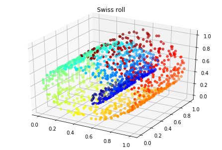
Suppose we have a set of data scattered in higher dimensions that we want to fit a multivariate normal distribution (Gaussian).
The arbitrary pdf of such data is:
$$p(x | \mu, \Sigma) = \frac{1}{( 2 \pi )^{D/2} | \Sigma |^{1/2}} \exp{\left ( -\frac{1}{2} (x-\mu)^{T} \Sigma^{-1} (x-\mu) \right )}$$
Where $x$ and $\mu$ are vectors and $\Sigma$ is a matrix better represented as: $\underline{x}, \underline{\mu}, \underline{\underline{\Sigma}}$. And $D$ is the dimensionality of our dataset.
Suppose we have a dataset $X$ such that:
$$X = \left [ x_1, x_2, x_3, \dots, x_N \right ]$$
This way we can rewrite the independent probabilities as:
$$p(X | \mu, \Sigma) = \prod_{i=1}^{N} p(x_{i} | \mu, \Sigma) = \prod_{i=1}^{N} \frac{1}{( 2 \pi )^{D/2} | \Sigma |^{1/2}} \exp{\left ( -\frac{1}{2} (x_{i}-\mu)^{T} \Sigma^{-1} (x_{i}-\mu) \right )}$$
Log likelihood
Due to the fact that we want to maximize/minimize, it is helpful to look at the log of the probabilities which simplifies the calculations.
$$L \left ( X | \mu, \Sigma \right ) = \log \left ( p(X | \mu, \Sigma) \right ) = -\frac{ND}{2} \log {2 \pi} - \frac{N}{2} \log{| \Sigma |} -\frac{1}{2} \sum_{i=1}^{N} (x_{i}-\mu)^{T} \Sigma^{-1} (x_{i}-\mu) $$
Mean estimation
To minimize the log likelihood function, we will set the derivative to zero. The partial derivative will look like this:
$$ \frac{\partial{L}}{\partial{\mu}} = \sum_{i=1}^{N} (x_i - \mu)^{T} \Sigma^{-1} = \left ( \nabla_{\mu} L \right )^{T}$$
Assuming that $\Sigma$ is invertible, setting this partial to zero gives us:
$$ \mu = \frac{1}{N} \sum_{i=1}^{N} x_i := \overline{x}$$
Math refresher
For this part we have to understand some properties of vector calculus that will be relevant.
Derivative of inverted matrix.
$$\partial{\Sigma^{-1}}$$
To compute this, we will refer back to the identity of invertible matrices.
$$\Sigma \Sigma^{-1} = I$$
Taking the derivative here gives:
$$\partial{\Sigma} \Sigma^{-1} + \Sigma \partial{\Sigma^{-1}} = 0 \rightarrow \partial{\Sigma^{-1}} = - \Sigma^{-1} \partial{\Sigma} \Sigma^{-1} $$
Derivative of determinants
With a proof by induction, we can show this for an arbitrary 2x2 matrix:
$$ \left |
\begin{matrix}
a(x) & b(x) \
c(x) & d(x)
\end{matrix}
\right | = a(x) d(x) - b(x) c(x)
$$
$$ \frac{d}{dx} \left |
\begin{matrix}
a(x) & b(x) \
c(x) & d(x)
\end{matrix}
\right | = a'(x) d(x) + a(x) d'(x) - b'(x) c(x) - b(x) c'(x)
$$
If we rearrange the terms by pairing every other term, we get:
$$\left [ a'(x) d(x) - b'(x) c(x) \right ] + \left [a(x) d'(x) - - b(x) c'(x) \right ] =
\left | \begin{matrix}
a'(x) & b'(x) \
c(x) & d(x)
\end{matrix} \right | +
\left | \begin{matrix}
a(x) & b(x) \
c'(x) & d'(x)
\end{matrix} \right |
$$
This is known as Jacobi's formula and the general formula goes like this:
$$\frac{d}{dt} \det{A(t)} = \det{A(t)} \cdot \textup{tr} \left ( A(t)^{-1} \cdot \frac{dA(t)}{dt} \right )$$
Where $\textup{tr}$ is the trace of the matrix.
The trace has a nice circular property such that $\textup{tr} (ABC) = \textup{tr}(CBA)$
NOTE the trace of a scalar is the same as itself. We can see that in the generalized quadratic form using matrix algebra.
$$f(x) = x^TAx = tr(x^TAx)$$
Derivative of multi-variate function with Taylor series
Suppose we have the vector valued function $f(\underline{x})$ that we wish to take the derivative of:
$$
f(x + \epsilon) = f(x) + \sum_{i} \sum_{j} \left( \frac{\partial f}{\partial x_{ij}} \epsilon_{ij} \right) + O(\epsilon^2)
$$
It turns out that in order to convert the output to the dimensionality required for the derivative, the combined partial sums of the derivative are equal to the trace:
$$
\sum_{i} \sum_{j} \left( \frac{\partial f}{\partial x_{ij}} \epsilon_{ij} \right) = \text{tr} \left( \left( \frac{\partial f}{\partial x} \right)^{T} \epsilon \right)
$$
Covariance estimation
Now that we have all the tools we need, we shall try to set the partial of the log likelihood with respect to the covariance to zero.
$$ \frac{\partial L}{\partial \Sigma} = - \frac{N}{2} \Sigma^{-1} - \frac{1}{2} \frac{\partial}{\partial \Sigma} \sum_{i=1}^{N} (x_{i}-\mu)^{T} \Sigma^{-1} (x_{i}-\mu) $$
By the derivative of multi-variate functions we know that the combined partial sums evaluate to the trace:
$$ \frac{\partial L}{\partial \Sigma} = - \frac{N}{2} \Sigma^{-1} - \frac{1}{2} \sum_{i=1}^{N} \textup{tr} \left ( (-1) (x_{i}-\mu)^{T} \Sigma^{-1} \Sigma^{-1} (x_{i}-\mu) \right )$$
We remember from the derivative of the inverse of a matrix and the circular trace result, we arrive at the following:
$$ \frac{\partial L}{\partial \Sigma} = - \frac{N}{2} \Sigma^{-1} - \frac{1}{2} \sum_{i=1}^{N} (-1) \Sigma^{-1} (x_{i}-\mu) (x_{i}-\mu)^{T} \Sigma^{-1}$$
Now we can set the derivative equal to zero:
$$N\Sigma^{-1} = \sum_{i=1}^{N} \Sigma^{-1} (x_{i}-\mu) (x_{i}-\mu)^{T} \Sigma^{-1}$$
Right multiply by $\Sigma$ to get:
$$ \Sigma = \frac{1}{N} \sum_{i=1}^{N} (x_{i}-\mu) (x_{i}-\mu)^{T}$$
Implementation
Here is the python code that computes the MLE for a given dataset:
from pprint import pprint

def mean_vector(data: list[list[float]]) -> list[float]:
    """
    Compute the mean vector of the data.

    Parameters:
    data (list of list of floats): A list of lists where each inner list is a data point.

    Returns:
    list of floats: The mean vector.
    """
    # Number of samples and features
    num_samples = len(data)
    num_features = len(data[0])

    # Initialize mean vector with zeros
    mean = [0] * num_features

    # Calculate the sum for each feature
    for i in range(num_samples):
        for j in range(num_features):
            mean[j] += data[i][j]

    # Compute the mean by dividing by the number of samples
    mean = [x / num_samples for x in mean]
    return mean

def covariance_matrix(data: list[list[float]], mean: list[float]) -> list[list[float]]:
    """
    Compute the covariance matrix of the data given the mean vector.

    Parameters
    ----------
    data: list[list[float]]
        A list of lists where each inner list is a data point.
    mean: list[float]
        The mean vector.

    Returns
    -------
    list[list[float]]
        The covariance matrix.
    """
    num_samples = len(data)
    num_features = len(data[0])

    # Initialize covariance matrix with zeros
    covariance = [[0] * num_features for _ in range(num_features)]

    # Compute the covariance matrix
    for i in range(num_features):
        for j in range(num_features):
            cov_sum = 0
            for k in range(num_samples):
                cov_sum += (data[k][i] - mean[i]) * (data[k][j] - mean[j])
            covariance[i][j] = cov_sum / (num_samples - 1)  # Use n-1 for sample covariance

    return covariance

# Example usage
data = [
    [2.5, 3.5, 4.5],
    [3.0, 3.0, 4.0],
    [2.0, 4.0, 5.0],
    [3.5, 3.5, 4.5],
    [3.0, 4.5, 5.5]
]

mean = mean_vector(data)
covariance = covariance_matrix(data, mean)

print("MLE Mean Vector:")
pprint(mean)
print("MLE Covariance Matrix:")
pprint(covariance)
MLE Mean Vector:
[2.8, 3.7, 4.7]
MLE Covariance Matrix:
[[0.325, -0.07499999999999998, -0.07499999999999998],
 [-0.07499999999999998, 0.32499999999999996, 0.32499999999999996],
 [-0.07499999999999998, 0.32499999999999996, 0.32499999999999996]]