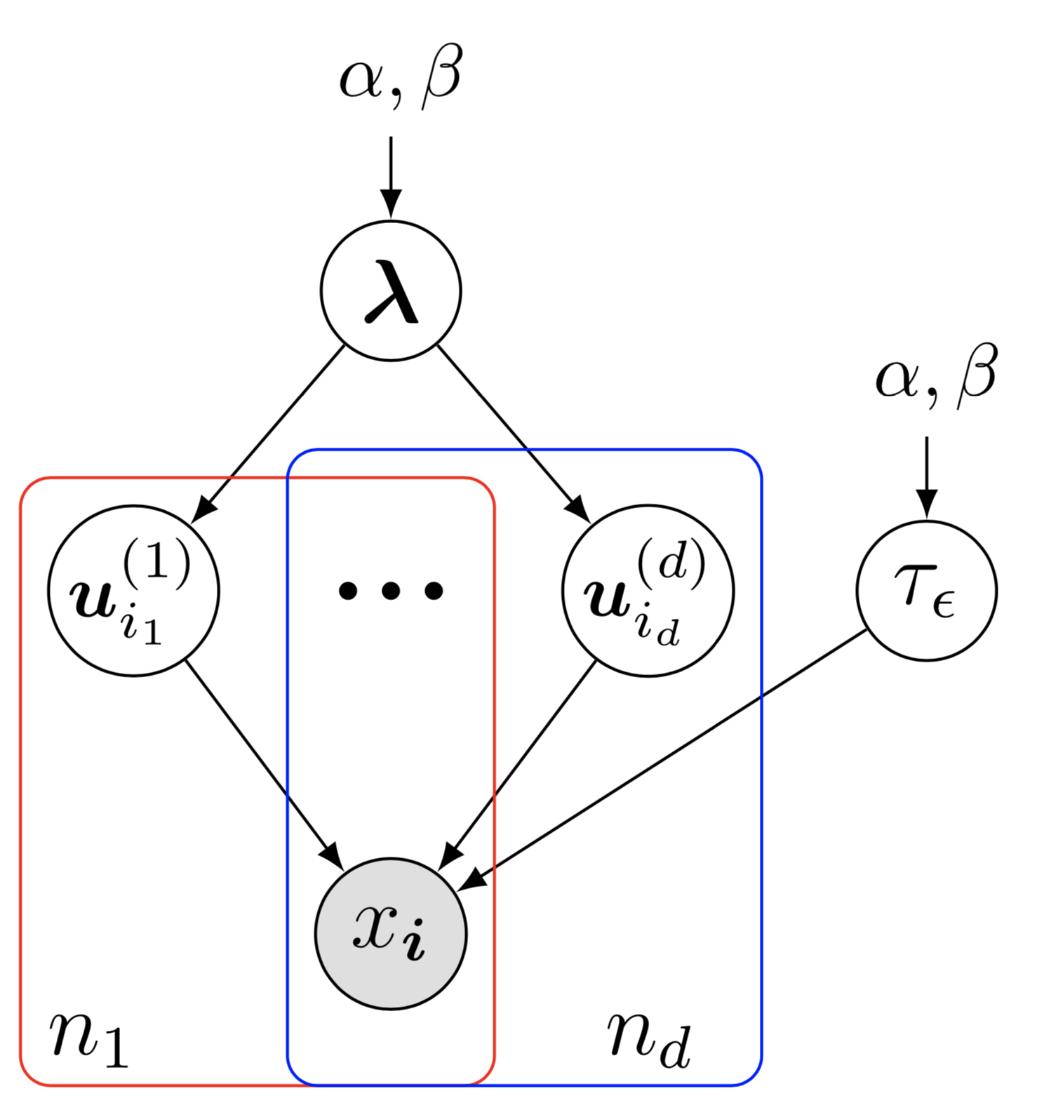
awesome-latex-drawing
Drawing Bayesian networks, graphical models, tensors, technical frameworks, and illustrations in LaTeX.
- 2.1k
- TeX
- MIT
- 18 mo ago
Temporal matrix factorization for sparse traffic time series forecasting.
Repo xinychen/tracebase, read from GitHub 1 min ago. xinychen has not joined Take My Repo.
xinychen/tracebase is a public repo on GitHub by xinychen. Temporal matrix factorization for sparse traffic time series forecasting. It declares the MIT license on GitHub. It is written mainly in Jupyter Notebook, has 59 stars and last changed on 2025-05-16. Nobody has reviewed it on Take My Repo yet, which says nothing about its quality. Read from GitHub on 2026-11-22.
Forecasting on high-dimensional and sparse Uber movement speed data of urban road networks with temporal matrix factorization techniques.
Uber movement project provides data and tools for cities to more deeply understand and address urban transportation problems and challenges. Uber movement speed data measure hourly street speeds across a city (e.g., New York City, Seattle, and London) to enable data-driven city planning and decision making. These data are indeed multivariate time series with N road segments and T time steps (hours), and are featured as high-dimensional, sparse, and nonstationary. To overcome the challenge created by these complicated data behaviors, we propose a temporal matrix factorization framework for multivariate time series forecasting on high-dimensional and sparse Uber movement speed data.
Uber movement project is not available now!
A detailed introduction to the analysis of missing data problem in Uber movement speed data is available on Medium.
speeds and one specific time period.
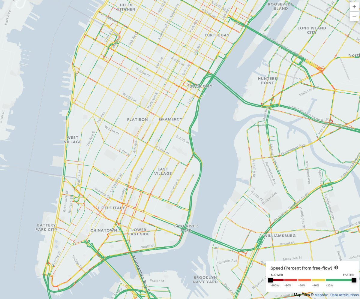
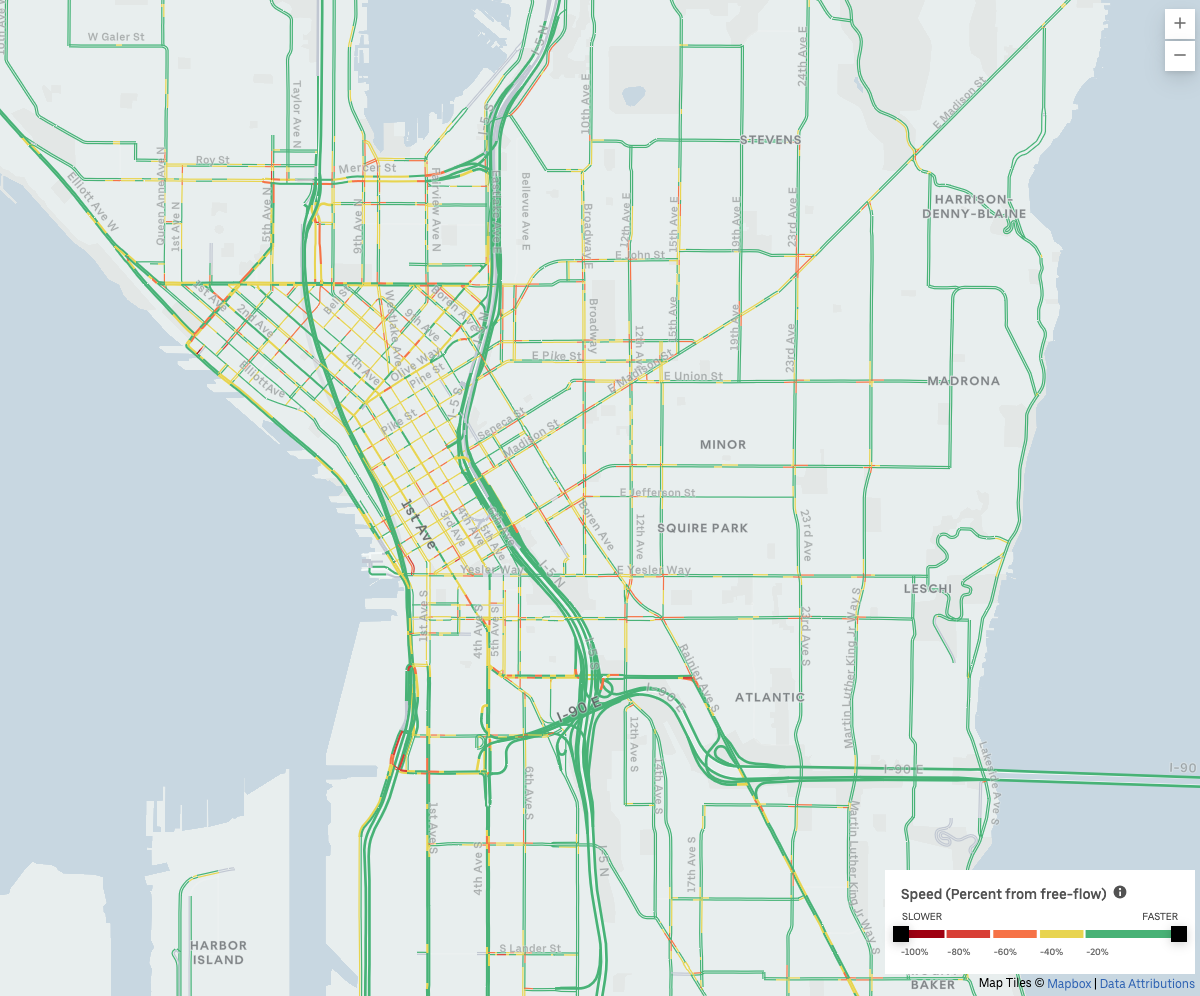
Figure 1: Uber movement speed heatmaps of New York City (left panel) and Seattle (right panel), USA.
Please download movement-speeds-hourly-new-york-2019-1.csv (movement speed data file of New York City in January 2019).
import pandas as pd
import numpy as np

data = pd.read_csv('movement-speeds-hourly-new-york-2019-1.csv')
road = data.drop_duplicates(['osm_way_id', 'osm_start_node_id', 'osm_end_node_id'])
road = road.drop(['year', 'month', 'day', 'hour', 'utc_timestamp', 'segment_id', 'start_junction_id',
                  'end_junction_id', 'speed_mph_mean', 'speed_mph_stddev'], axis = 1)
road.to_csv('road.csv')
In New York City, Uber movement project covers 98,210 road segments.
This process is time-consuming.
import numpy as np
import pandas as pd

month = 1
data = pd.read_csv('movement-speeds-hourly-new-york-2019-{}.csv'.format(month))
road = pd.read_csv('road.csv')
tensor = np.zeros((road.shape[0], max(data.day.values), 24))
k = 0
for i in range(road.shape[0]):
    temp = data[(data['osm_way_id'] == road.osm_way_id.iloc[i])
                & (data['osm_start_node_id'] == road.osm_start_node_id.iloc[i])
                & (data['osm_end_node_id'] == road.osm_end_node_id.iloc[i])]
    for j in range(temp.shape[0]):
        tensor[k, temp.day.iloc[j] - 1, temp.hour.iloc[j]] = temp.speed_mph_mean.iloc[j]
    k += 1
    if (k % 1000) == 0:
        print(k)
mat = tensor.reshape([road.shape[0], max(data.day.values) * 24])
np.savez_compressed('hourly_speed_mat_2019_{}.npz'.format(month), mat)

del data, tensor
The matrix's row corresponds to one specific road segment, while the column corresponds to one specific hour.
In this repository, we prepare the dataset and place it at the folder datasets/NYC-movement-data-set:
hourly_speed_mat_2019_1.npz (91 MB): data is of size 98,210 x 744 with 23,228,581 positive speed observations.hourly_speed_mat_2019_2.npz (85.2 MB): data is of size 98,210 x 672 with 21,912,460 positive speed observations.hourly_speed_mat_2019_3.npz (38.1 MB): data is of size 98,210 x 264 with 10,026,045 positive speed observations.Note that to make the data as small as possible, we only maintain the data during the first 11 days of March 2019, and save it as hourly_speed_mat_2019_3.npz. You can use the following code to drop the unnecessary portion when preprocessing the raw data.
month = 3
data = pd.read_csv('movement-speeds-hourly-new-york-2019-{}.csv'.format(month))
road = pd.read_csv('road.csv')
i = data[(data.day > 11)].index
data = data.drop(i)
You can also consider to use the prepared Seattle Uber movement speed data at the folder datasets/Seattle-movement-data-set:
hourly_speed_mat_2019_1.npz (26.4MB)hourly_speed_mat_2019_2.npz (25.2MB)hourly_speed_mat_2019_3.npz (31.6MB)If you want to investigate the missing data problem in Uber movement speed data, please prepare the data in the whole year of 2019 by yourself through the above codes. You can also skip this part and check out our documentation for multivariate time series forecasting on NYC Uber movement speed dataset in the next part.
## Build a speed matrix for the whole year of 2019 in NYC
mat = np.load('hourly_speed_mat_2019_1.npz')['arr_0']
for month in range(2, 13):
    mat = np.append(mat, np.load('hourly_speed_mat_2019_{}.npz'.format(month))['arr_0'], axis = 1)

## Calculate missing rates
print('The missing ratte of speed matrix is:')
print(len(np.where(mat == 0)[0]) / (mat.shape[0] * mat.shape[1]))

N, T = mat.shape
sample_rate = np.zeros(T)
for t in range(T):
    pos = np.where(mat[:, t] == 0)
    sample_rate[t] = len(pos[0]) / N
sample_rate = sample_rate[: 52 * 7 * 24].reshape([52, 24 * 7])
whole_rate = np.mean(sample_rate, axis = 0)
rate = len(np.where(mat == 0)[0]) / (mat.shape[0] * mat.shape[1])
print(rate)
import matplotlib.pyplot as plt

plt.rcParams['font.size'] = 12
fig = plt.figure(figsize = (8, 2))
ax = fig.add_subplot(1, 1, 1)
plt.plot(whole_rate, color = 'red', linewidth = 1.8)
upper = whole_rate + np.std(sample_rate, axis = 0)
lower = whole_rate - np.std(sample_rate, axis = 0)
x_bound = np.append(np.append(np.append(np.array([0, 0]), np.arange(0, 7 * 24)),
                              np.array([7 * 24 - 1, 7 * 24 - 1])), np.arange(7 * 24 - 1, -1, -1))
y_bound = np.append(np.append(np.append(np.array([upper[0], lower[0]]), lower),
                              np.array([lower[-1], upper[-1]])), np.flip(upper))
plt.fill(x_bound, y_bound, color = 'red', alpha = 0.2)
plt.axhline(y = rate, color = 'gray', alpha = 0.5, linestyle='dashed')
plt.xticks(np.arange(0, 24 * 7 + 1, 1 * 24))
plt.xlabel('Time (hour)')
plt.ylabel('Missing rate')
plt.grid(axis = 'both', linestyle = 'dashed', linewidth = 0.1, color = 'gray')
ax.tick_params(direction = 'in')
ax.set_xlim([-1, 7 * 24])
# ax.set_ylim([0.6, 1])
plt.show()
# fig.savefig('NYC_missing_rate_stat.pdf', bbox_inches = 'tight')


Figure 2: The missing rates of Uber movement speed data aggregated per week over the whole year of 2019. The red curve shows the aggregated missing rates in all 52 weeks. The red area shows the standard deviation of missing rates in each hour over 52 weeks. The 168 time steps refer to 168 hours of Tuesday, Wednesday, Thursday, Friday, Saturday, Sunday, and Monday. (Left panel) The dataset has 98,210 road segments, and the whole missing rate is 64.43%. (Right panel) The dataset has 63,490 road segments, and the whole missing rate is 84.95%.
import numpy as np

mat = np.load('hourly_speed_mat_2019_1.npz')['arr_0']
for month in range(2, 13):
    mat = np.append(mat, np.load('hourly_speed_mat_2019_{}.npz'.format(month))['arr_0'], axis = 1)
ratio = np.sum(mat > 0, axis = 1) / (365 * 24)
Print observation rate results:
for threshold in 0.1 * np.arange(1, 10):
    print('Observation rate > {0:.2f}'.format(threshold))
    print(np.sum(ratio > threshold))
    print(np.sum(ratio > threshold) / ratio.shape[0])
    print()
In this research, we aim at simultaneously handling the following emerging issues in real-world time series datasets: 1) High-dimensionality (i.e., large $N$): data is of large scale with thousands of multivariate variables. 2) Sparsity and missing values: data is incomplete with missing values, and sometime only a small fraction of data is observed due to the data collection mechanism. 3) Nonstationarity: real-world time series often show strong seasonality and trend. For instance, the Uber movement speed dataset registers traffic speed data from thousands of road segments with strong daily and weekly periodic patterns. And due to insufficient sampling and limited penetration of ridesharing vehicles, we only have access to a small fraction of observed value even in hourly resolution.

Figure 3: Illustration of the multivariate time series forecasting task on the incomplete data $\{\boldsymbol{y}_{1},\boldsymbol{y}_{2},\ldots,\boldsymbol{y}_{T}\}$. Note that the time series are high-dimensional, sparse, and nonstationary.
The temporal matrix factorization consists of matrix factorization (on partially observed time series) and vector autoregressive (VAR) process (on temporal factors).

Figure 4: Illustration of TMF on multivariate time series data. For spatiotemporal traffic states data, it can be factorized into spatial factors and temporal factors in which the temporal factor matrix is indeed a multivariate time series. We aim to impose a certain temporal modeling structure on temporal factor matrix.
We evaluate the proposed model mainly on the Uber movement speed data because these time series data are featured as high-dimensional and sparse. The rolling forecasting scenario is illustrated as follows.

Figure 5: Illustration of the rolling forecasting scenario on multivariate time series data $\{\boldsymbol{y}_1,\boldsymbol{y}_2,\ldots,\boldsymbol{y}_9\}$. This example shows that the forecasting time horizon is 2, and what we need to forecast includes $\{\boldsymbol{y}_{4},\boldsymbol{y}_{5},\boldsymbol{y}_{6},\boldsymbol{y}_{7},\boldsymbol{y}_{8},\boldsymbol{y}_{9}\}$.
We implement our algorithms with NumPy library, possibly being easy for understanding each line. It should be no barrier for running these codes on any Python environment with a NumPy library. If you have any questions, feel free to create an issue in this repository. If you are looking for an intuitive explanation, please check out our blog post temporal matrix factorization for multivariate time series forecasting on Medium.
Our Python implementation with
numpycan be adapted to a GPU implementation withcupy, please replaceimport numpy as npbyimport cupy as np. It would be not difficult to follow the experiment.
def compute_mape(var, var_hat):
    return np.sum(np.abs(var - var_hat) / var) / var.shape[0]

def compute_rmse(var, var_hat):
    return np.sqrt(np.sum((var - var_hat) ** 2) / var.shape[0])
def generate_Psi(T, d, season):
    Psi = []
    for k in range(0, d + 1):
        if k == 0:
            Psi.append(np.append(np.zeros((T - d - season, d)),
                                 np.append(-1 * np.eye(T - d - season), np.zeros((T - d - season, season)), axis = 1)
                                 + np.append(np.zeros((T - d - season, season)), np.eye(T - d - season), axis = 1), axis = 1))
        else:
            Psi.append(np.append(np.append(np.zeros((T - d - season, d - k)),
                                           np.append(-1 * np.eye(T - d - season), np.zeros((T - d - season, season)), axis = 1)
                                           + np.append(np.zeros((T - d - season, season)), np.eye(T - d - season), axis = 1), axis = 1),
                                 np.zeros((T - d - season, k)), axis = 1))
    return Psi
This is a classical approach for defining temporal operators, one effective alternative is defining these temporal operators as sparse arrays in both numpy and cupy. Please check out How to define temporal operators as sparse arrays in both numpy (for CPU) and cupy (for GPU)?
For an intuitive explanation, please check out using conjugate gradient to solve matrix equations.
def update_cg(var, r, q, Aq, rold):
    alpha = rold / np.inner(q, Aq)
    var = var + alpha * q
    r = r - alpha * Aq
    rnew = np.inner(r, r)
    q = r + (rnew / rold) * q
    return var, r, q, rnew

def ell_w(ind, W, X, rho):
    return X @ ((W.T @ X) * ind).T + rho * W

def conj_grad_w(sparse_mat, ind, W, X, rho, maxiter = 5):
    rank, dim1 = W.shape
    w = np.reshape(W, -1, order = 'F')
    r = np.reshape(X @ sparse_mat.T - ell_w(ind, W, X, rho), -1, order = 'F')
    q = r.copy()
    rold = np.inner(r, r)
    for it in range(maxiter):
        Q = np.reshape(q, (rank, dim1), order = 'F')
        Aq = np.reshape(ell_w(ind, Q, X, rho), -1, order = 'F')
        w, r, q, rold = update_cg(w, r, q, Aq, rold)
    return np.reshape(w, (rank, dim1), order = 'F')

def ell_x(ind, W, X, A, Psi, d, lmbda, rho):
    rank, dim2 = X.shape
    temp = np.zeros((d * rank, Psi[0].shape[0]))
    for k in range(1, d + 1):
        temp[(k - 1) * rank : k * rank, :] = X @ Psi[k].T
    temp1 = X @ Psi[0].T - A @ temp
    temp2 = np.zeros((rank, dim2))
    for k in range(d):
        temp2 += A[:, k * rank : (k + 1) * rank].T @ temp1 @ Psi[k + 1]
    return W @ ((W.T @ X) * ind) + rho * X + lmbda * (temp1 @ Psi[0] - temp2)

def conj_grad_x(sparse_mat, ind, W, X, A, Psi, d, lmbda, rho, maxiter = 5):
    rank, dim2 = X.shape
    x = np.reshape(X, -1, order = 'F')
    r = np.reshape(W @ sparse_mat - ell_x(ind, W, X, A, Psi, d, lmbda, rho), -1, order = 'F')
    q = r.copy()
    rold = np.inner(r, r)
    for it in range(maxiter):
        Q = np.reshape(q, (rank, dim2), order = 'F')
        Aq = np.reshape(ell_x(ind, W, Q, A, Psi, d, lmbda, rho), -1, order = 'F')
        x, r, q, rold = update_cg(x, r, q, Aq, rold)
    return np.reshape(x, (rank, dim2), order = 'F')
notmf).def notmf(dense_mat, sparse_mat, rank, d, lmbda, rho, season, maxiter): dim1, dim2 = sparse_mat.shape W = 0.01 * np.random.randn(rank, dim1) X = 0.01 * np.random.randn(rank, dim2) A = 0.01 * np.random.randn(rank, d * rank) if np.isnan(sparse_mat).any() == False: ind = sparse_mat != 0 pos_test = np.where((dense_mat != 0) & (sparse_mat == 0)) elif np.isnan(sparse_mat).any() == True: pos_test = np.where((dense_mat != 0) & (np.isnan(sparse_mat))) ind = ~np.isnan(sparse_mat) sparse_mat[np.isnan(sparse_mat)] = 0 dense_test = dense_mat[pos_test] del dense_mat Psi = generate_Psi(dim2, d, season) show_iter = 100 temp = np.zeros((d * rank, dim2 - d - season)) for it in range(maxiter): W = conj_grad_w(sparse_mat, ind, W, X, rho) X = conj_grad_x(sparse_mat, ind, W, X, A, Psi, d, lmbda, rho) for k in range(1, d + 1): temp[(k - 1) * rank : k * rank, :] = X @ Psi[k].T A = X @ Psi[0].T @ np.linalg.pinv(temp) mat_hat = W.T @ X if (it + 1) % show_iter == 0: temp_hat = mat_hat[pos_test] print('Iter: {}'.format(it + 1)) print('MAPE: {:.6}'.format(compute_mape(dense_test, temp_hat))) print('RMSE: {:.6}'.format(compute_rmse(dense_test, temp_hat))) print() return mat_hat, W, X, A def notmf_dic(obs, W, X, A, d, lmbda, rho, season): dim1, dim2 = obs.shape rank = X.shape[0] if np.isnan(obs).any() == False: ind = obs != 0 elif np.isnan(obs).any() == True: ind = ~np.isnan(obs) obs[np.isnan(obs)] = 0 Psi = generate_Psi(dim2, d, season) X = conj_grad_x(obs, ind, W, X, A, Psi, d, lmbda, rho) temp = np.zeros((d * rank, dim2 - d - season)) for k in range(1, d + 1): temp[(k - 1) * rank : k * rank, :] = X @ Psi[k].T A = X @ Psi[0].T @ np.linalg.pinv(temp) return X, A
def var4cast(X, A, d, delta, season):
    dim1, dim2 = X.shape
    X_hat = np.append(X[:, season:] - X[:, : -season], np.zeros((dim1, delta)), axis = 1)
    for t in range(delta):
        X_hat[:, dim2 - season + t] = A @ X_hat[:, dim2 - season + t - np.arange(1, d + 1)].T.reshape(dim1 * d)
    X = np.append(X, np.zeros((dim1, delta)), axis = 1)
    for t in range(delta):
        X[:, dim2 + t] = X[:, dim2 - season + t] + X_hat[:, dim2 - season + t]
    return X
from ipywidgets import IntProgress
from IPython.display import display

def rolling4cast(dense_mat, sparse_mat, pred_step, delta, rank, d, lmbda, rho, season, maxiter):
    dim1, T = sparse_mat.shape
    start_time = T - pred_step
    max_count = int(np.ceil(pred_step / delta))
    mat_hat = np.zeros((dim1, max_count * delta))
    f = IntProgress(min = 0, max = max_count) # instantiate the bar
    display(f) # display the bar
    for t in range(max_count):
        if t == 0:
            _, W, X, A = notmf(dense_mat[:, : start_time], sparse_mat[:, : start_time],
                               rank, d, lmbda, rho, season, maxiter)
        else:
            X, A = notmf_dic(sparse_mat[:, : start_time + t * delta], W, X_new, A, d, lmbda, rho, season)
        X_new = var4cast(X, A, d, delta, season)
        mat_hat[:, t * delta : (t + 1) * delta] = W.T @ X_new[:, - delta :]
        f.value = t
    small_dense_mat = dense_mat[:, start_time : T]
    pos = np.where((small_dense_mat != 0) & (np.invert(np.isnan(small_dense_mat))))
    mape = compute_mape(small_dense_mat[pos], mat_hat[pos])
    rmse = compute_rmse(small_dense_mat[pos], mat_hat[pos])
    print('Prediction MAPE: {:.6}'.format(mape))
    print('Prediction RMSE: {:.6}'.format(rmse))
    print()
    return mat_hat, W, X, A
import numpy as np

dense_mat = np.load('../datasets/NYC-movement-data-set/hourly_speed_mat_2019_1.npz')['arr_0']
for month in range(2, 4):
    dense_mat = np.append(dense_mat, np.load('../datasets/NYC-movement-data-set/hourly_speed_mat_2019_{}.npz'.format(month))['arr_0'], axis = 1)

import time
for rank in [10]: # rank of matrix factorization
    for delta in [1, 2, 3, 6]: # forecasting time horizon
        for d in [6]: # order of VAR
            start = time.time()
            pred_step = 7 * 24
            lmbda = 1
            rho =  5
            season = 7 * 24
            maxiter = 50
            mat_hat, W, X, A = rolling4cast(dense_mat[:, : 24 * 7 * 10], dense_mat[:, : 24 * 7 * 10],
                                            pred_step, delta, rank, d, lmbda, rho, season, maxiter)
            print('delta = {}'.format(delta))
            print('rank R = {}'.format(rank))
            print('Order d = {}'.format(d))
            end = time.time()
            print('Running time: %d seconds'%(end - start))
Tracebase provides a collection of time series forecasting approaches and algorithms for you. We aim to support you to explore traffic flow data in urban areas with machine learning models. We provide friendly implementation with a few lines relying on pandas and numpy packages.
or
@article{chen2025nonstationary,
  title={Forecasting sparse movement speed of urban road networks with nonstationary temporal matrix factorization},
  author={Chen, Xinyu and Zhang, Chengyuan and Zhao, Xi-Le and Saunier, Nicolas and Sun, Lijun},
  journal={Transportation Science},
  year={2025}
}

@article{chen2024forecasting,
  title={Forecasting urban traffic states with sparse data using Hankel temporal matrix factorization},
  author={Chen, Xinyu and Zhao, Xi-Le and Cheng, Chun},
  journal={INFORMS Journal on Computing},
  year={2024}
}Data retrieved from Uber Movement, © 2022 Uber Technologies, Inc., https://movement.uber.com.


xinychen/tracebase is a public repo on GitHub by xinychen. Temporal matrix factorization for sparse traffic time series forecasting.
It declares the MIT license on GitHub.
Its maker has not tagged a system, so it is unknown here. Its README says what it needs.
Open "Take it" on its page: Take My Repo writes an install plan for your machine and hands it to your AI agent (Claude Code, Codex or Cursor), which asks you before each step. Take My Repo has not tested it on any machine.
Its last change on GitHub was on 2025-05-16. GitHub counts 2 open issues and pull requests. Take My Repo does not judge from that whether it is maintained.
Nobody has reviewed it on Take My Repo yet, which says nothing about its quality.
Drawing Bayesian networks, graphical models, tensors, technical frameworks, and illustrations in LaTeX.
LaTeX论文写作教程 (清华大学出版社)
Machine learning for transportation data imputation and prediction.
Tensor decomposition for machine learning (w/ Python implementation)
Providing codes (including Matlab and Python) for visualizing numerical experiment results.